The Central Limit Theorem has a unique importance in the field of data science. In fact, many believe it’s one of the few theorems data scientists need to know.
Early version of the Central Limit Theorem was discovered as far back as 1733 by Abraham de Moivre. Today, it continues to be applied to a great extent, especially in data science and machine learning algorithms.
In this article, we will learn the theorem of central limit, how it works, and why it’s so useful in data science and analytics.
What is the Central Limit Theorem
To understand what is the central limit theorem, we must begin by looking at the central limit theorem definition. Although there is no one complete central limit definition, here is the one commonly found in most statistics textbooks.
“The Central Limit Theorem (CLT) is a statistical theory states that given a sufficiently large sample size from a population with a finite level of variance, the mean of all samples from the same population will be approximately equal to the mean of the population.”
This Central Limit Theorem definition does not quite explain the meaning and purpose of the theorem to a layperson. But the CLT is actually fairly easy to understand. It simply says that with large sample sizes, the sample means are normally distributed. To understand this better, we first need to define all the terms.
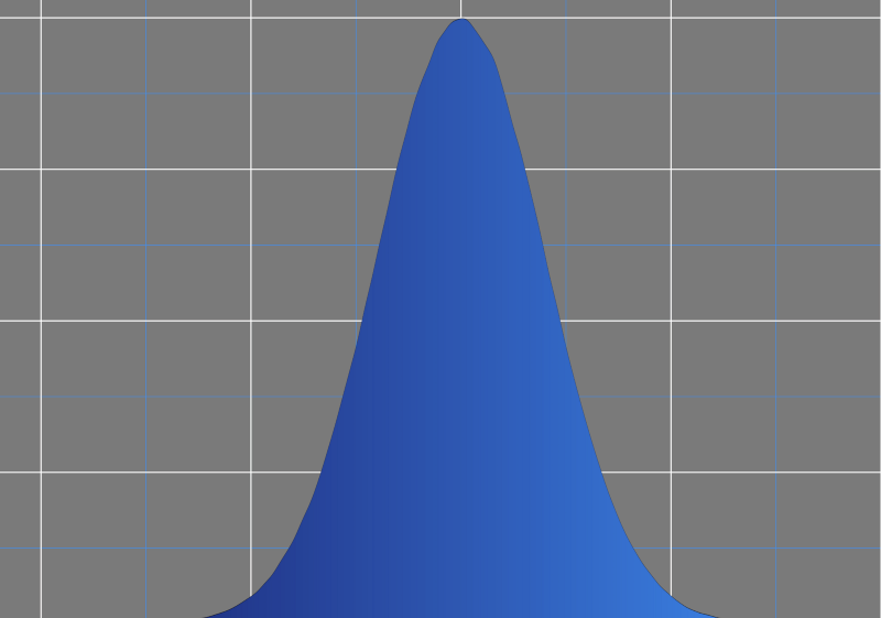
A normal distribution simply means that a set of numbers, when mapped on a graph, would look like a bell curve. In other words, there are fewer numbers at the two extremes and most of the numbers are clustered around the average.
A Normal Distribution
Sample Mean
The sample mean is the average of a subset of a larger dataset where the subset data is chosen at random. For instance, if you randomly picked 15 students out of a class of 150 students and noted their ages. The average age of those 15 students would be the sample mean. Obviously, since the sample is chosen randomly, the sample mean would be different every single time.
Since the central limit theorem definition talks about large sample sizes, we need to define what constitutes a large sample. Although this is subjective of course, by and large, a sample size above 30 is considered to be a large sample. Of course, depending on the actual context, the sample may need to be a lot larger.
In other words, the Central Limit Theorem simply states that if you have 30 or more data points in your sample. According to the statement, the mean of that sample will be part of a bell-shaped curve.
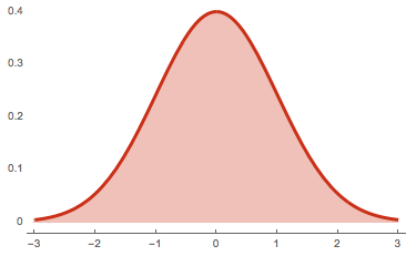
Therefore, if you had a number of large samples and plotted their means, it would be a bell-shaped curve as seen in the graph above. In other words, most of the sample means would be closer to the center with a few averages lying on either extreme.
Of course, it’s important to remember that the Central Limit Theorem only says that the sample means of the data will be normally distributed. It doesn’t make any similar assumptions about the distribution of the underlying data. In other words, it doesn’t claim that the age of all the students will be normally distributed as well.
How does the Central Limit Theorem work
In order to illustrate the working of the Central Limit Theorem, let’s look at a basic Central Limit Theorem example.
Suppose we have a population data with mean µ and standard deviation σ. Now, we select a random sample of data of size n (x1, x2, x3, … xn — 1, xn) from this population data.
We then repeat this process and select many such random samples from the population data as we can. Next, we calculate the mean or x̄ of every sample.
Now we need to examine the distribution of all the x̄ values. This is known as the sampling distribution of the mean (x̄). Here’s how the Central Limit Theorem works:
Given a distribution whose means is μ and variance(square of standard deviation) σ2. The sampling distribution of the mean will approach a normal distribution which has a mean μ and a variance σ2/n. As the value of n, which is the sample size, goes up.
As n increases, the normal distribution is reached very quickly. Many people tend to confuse n as the number of samples. It needs to be remembered that it is, in fact, the number of data points in each sample. In fact, in the sampling distribution of the mean, the number of samples is assumed to be infinite.
It’s important to remember that three major components form part of the Central Limit Theorem:
(i) Population distribution
(ii) An increasing sample size
(iii) Successive samples selected randomly from the population
This video describes the basics of the Central Limit Theorem and how it works.
How is Central Limit Theorem applied in Data Science & Machine Learning
One of the fundamental goals of any data analysis technique is hypothesis testing. The basic question behind every hypothesis test is “does the data support my hypothesis or would I get the same data even if my idea was completely wrong?”
In other words, you need to quantify the likelihood that you’re seeing the data due to chance and not due to your hypothesis. To understand the likelihood of seeing the same data even if your hypothesis is wrong. You first need to craft the range of values that you would see if your hypothesis was indeed wrong.
You then need to assess the likelihood of the observed data in such a scenario. This is where the Central Limit Theorem comes in. We use the Central Limit theorem example to illustrate how.
Central Limit Theorem Example
Let’s use a real-world data analysis problem to illustrate the utility of the Central Limit Theorem. Say a data scientist at a tech startup has been asked to figure out how engaging their homepage is.
As the first step, she has to decide which metric to use as a measure of engagement. She zeroes in on time spent on the homepage. This leads to the hypothesis that the homepage is engaging if the average time spent on it is over 7 minutes.
For the sake of practicality, she takes a sample of 10% of users over a period of 1 week to measure the time spent on the home page. Say the answer comes to 8.2 minutes. However, since this is a random sample, the average will vary with every sample that is selected.
To confirm that the answer of 8.2 minutes actually reflects the engagement with the website. She now has to assess the likelihood that the result is due to chance. Or, how likely is it that the actual engagement rate of the population is below 7 minutes and the result of 8.2 minutes is only due to a random chance?
Results
In such a case, as long as the sample size is more than 30. The Central Limit Theorem can be used to construct the distribution of time spent on the homepage assuming the true average time spent is less than 7 minutes. This is known as the null distribution.
According to the Central Limit Theorem, the null distribution will be a normal distribution. The theorem also states that you can use values from the sample to approximate the values needed to create the null distribution. The middle of the null distribution is the mean of the null hypothesis.
Similarly, the standard deviation of the null distribution is the standard deviation of the sample divided by the square root of the sample size.
Once you prepare the null distribution, you plot the observed value, 8.2. Against the distribution to see how likely you would be to see the same value even if the engagement was under 7 minutes. The data would look something like this:
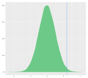
Distribution of Sample Means of Time on Homepage
The area of the distribution on the right of the blue line refers to the probability of observing a data point of 8.2 minutes when the true average is 7 minutes. Since this probability is sufficiently small, it is safe to say that it is extremely likely that the overall time spent on the homepage is indeed more than 7 minutes.
Conclusion
The Central Limit Theorem and the Bayes’ Theorem are probably the only theorems you’ll need to know inside out to master data science. The Central Limit Theorem helps you conduct hypothesis testing, which lies at the heart of any effective data analysis model. However, this is only one of the many mathematical concepts that are used extensively in data science. If you would like a career in data science or analytics, then a comprehensive course with live sessions, assessments, and placement assistance might be your best bet.