Introduction
Programming is an intrinsically difficult activity. Just like “there is no royal road to geometry”, likewise there is no royal road to data structures. Though each programming language is different but there are some dimensions where their data structures can be related and differentiate easily. For example, low-level versus high-level, general versus specific task domain, interpreted versus compiled, and so on. Python is a general-purpose programming language and it is relatively simple and easy to learn. In addition, it provides the kind of run time feedback which will help the novice programmers.
Just like any other programming language, data structure and algorithms in Python are its basic building blocks. Let us understand the basic data structures first and then we will learn about abstract data types. Hence, in the end, we would cover algorithms and know why they are important.
Note- If you really want to learn from this post then reading is not enough. At the very least you should try running some snippets in the post. And if you are completely new, know how to install python.
Basic Data Structures
Data Structure and Algorithms are building blocks of Python. It works in a similar manner as grammar works for high-level language. To get a more clear idea, follow comments in the snippets. For any queries related to the blog post, you can reach me in the comment section. Let’s start covering the topics on data structures and algorithms in Python.
List
List in Python is the same as ‘array’ in other languages. In addition, Python lists are heterogeneous, which means you can add any kind of value in a list. This can be string, numerical, a boolean, or even a list itself.
listA = [1,2,3,4,5]                 #Create list using square braces []

listA.extend([6,7])                 #Extend the list
print(list)

listA.append([8,9])                 #Append elements to the list
print(list)

listB = [10,11,12]                  #Create another list

listoflist = [listA, listB]         #Join two lists
print(listoflist)                   #Print
Tuples
# indexing is from 0
# Same as list apart from tuples are immutable, which means you can not change the content once the tuple is created.
# Use () instead of []

tuple = (2, 4, 6, 7)

#print length of tuple
print(len(tuple))

#print element at index 2
print(tuple[2])

#just like lists you can merge tuples too
a = (1, 2, 3)
b = (4, 5, 6)
merge = (a, b)
print(merge)
Dictionary
Dictionary needs a little introduction. In Python programming, the dictionary stores the information with the help of a unique key. Whenever you need that data, call it by the key it was assigned. Here the key is ‘ship1’, ‘ship2’ and the values are the name of captains.
#create the dictionary
captains = {}

#add values into it
captains["ship1"] = "Kirk"
captains["ship2"] = "Marcus"
captains["ship3"] = "Phillips"
captains["ship4"] = "Mike"

#fetch the data
#two ways to fetch the result from dictionary
print (captains["ship3"])
print (captains.get("ship4"))
Abstract Data Types(ADT)
Those which we saw above are inbuilt or pre-defined data types. So, now what is Abstract Data Type? ADT is defined as a data type that specifies a set of data values and a collection of well-defined operation. These data types can be performed on values.
ADT are defined independent of their implementation. They allow us to focus on the use of the new data type instead of how it’s implemented. This separation is typically enforced by requiring interaction with the abstract data type. The above interaction is obtained by an interface or defined set of operations, known as information hiding. By doing this, we can work with an abstraction and focus on what functionality the ADT provides instead of how that functionality is implemented.
Abstract data types can be viewed as black boxes as illustrated in figure. User programs interact with instances of the ADT by invoking one of the several operations defined by its interface. The set of operations can be grouped into four categories:
Constructors: Create and initialize new instances of the ADT
Accessors: Return data contained in an instance without modifying it.
Mutators: Modify the contents of an ADT instance
Iterators: Process individual data components sequentially.
To know more about ADT you can download data structures and algorithms in Python pdf by Necasie, everything explained there is worth reading.
Algorithms: how to use it for optimum data structure?
The most important thing to think about when designing and implementing a program is that its produced results can be relied upon. We want our bank balances to be calculated correctly and the fuel injectors in our automobiles to inject appropriate amounts of fuel. The preference is that neither airplanes nor operating systems crash. Isn’t it? That is why Algorithms and data structures in Python are important.
Thinking about Computational Complexity
How should one go about answering the question “How long will any single function take to run?” We could run the program on some input and time. Anyways, that wouldn’t be particularly informative because the result would depend upon the speed of the computer and the efficiency of the Python implementation and the value of input.
To simplify, we will use a more abstract measure of time. We measure time in terms of the number of basic steps executed by the program instead of measuring it in milliseconds. Now, the value of input, of course, the actual running time of an algorithm depends upon the size of the input and its values. Let’s take an example to understand this better. Consider a linear search algorithm implemented as under.
def linearSearch(L, x):
    for e in L:
        if e == x:
            return True
        return False
Justification
- Suppose that L is a list containing a million elements, and consider the call linear search(L, 3).
- If the first element in L is 3, it will return True almost immediately.
- On the other hand, if 3 is not in L, linear search will have to examine all one million elements before returning false.
- So, in general, there are three broad cases to think about:
The best-case running time is when the inputs of the algorithm are favorable up to their best. Similarly, the worst-case running time is the maximum running time over all the possible inputs of a given size. Finally, by the analogy with the definitions of the best and worst-case running time, the average-case running time is when all possible inputs of a given size.
This was the walk in the park( easy stuff), but sit tight as what we will walk through now is something like a Jurassic Park.
Asymptotic Notation
Analysis is derived from the relation between the running time of an algorithm and the size of its inputs. This procedure leads us to use the following rules of thumb in describing the asymptotic complexity of an algorithm.
If the running time is the sum of multiple terms, keep the one with the largest growth rate, and drop the others.
The most commonly used asymptotic notation is called ”Big O” notation and it is used to give an upper bound on the asymptotic growth of a function. We, like many computer scientists, will often abuse Big O notation by marking statements like, “the complexity of f(x) is O(x2).” By this, we mean that in the worst-case f will take O(x2) steps to run.
However, the difference between a function being “in O(x2)” and “being O(x2)” is subtle but important. When we say that f(x) is O(x2), we are implying that x2 is both an upper bound and a lower bound on the asymptotic worst-case running time. This is often called the tight-bound.
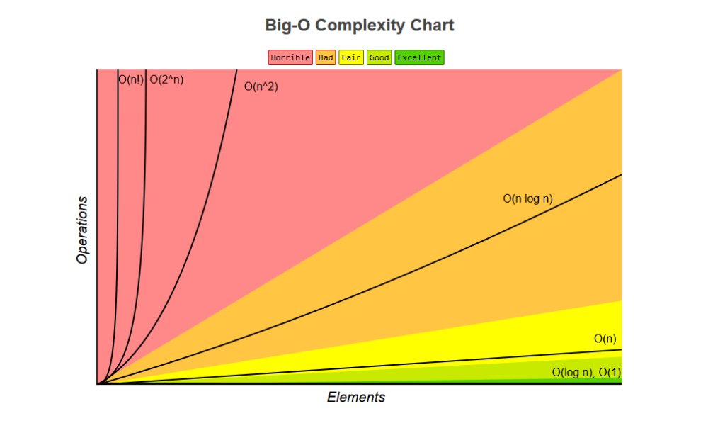
Some Important Complexity Classes
Some of the most common instances of Big O are listed below. In each case, n is a measure of the size of the inputs to the function.
O(1) denotes constant running time
O(log n) denotes logarithmic running time
O(n) denotes linear running time
O(n log n) denotes log-linear running time
O(nk) denotes polynomial running time. K is constant.
O(cn) denotes exponential running time. N is constant.
Simple Algorithm for illustration
Object-oriented data structures are very important in Python language. Let’s take a look at a simple search algorithm and you will get a better understanding of its working. A search algorithm is a method for finding an item or group of items of specific properties within a collection. We will be keeping Binary Search because it searches a sorted array. We will do this by dividing the search interval in half and ignore half of the elements just after one comparison. The procedure is simple,
- Compare x with the middle element.
- If x matches with middle element, we return the mid index.
- Else If x is greater than the mid element, then x can only lie in right half subarray after the mid element. So we recur for the right half.
- Else (x is smaller) recur for the left half.
Below is the Python implementation of Recursive Binary Search.
# Python Program for recursive binary search.

# Returns index of x in arr if present, else -1
def binarySearch (arr, l, r, x):

     # Check base case
     if r >= l:

              mid = l + (r - l)/2

              # If element is present at the middle itself
              if arr[mid] == x:
              return mid

             # If element is smaller than mid, then it
            # can only be present in left subarray
            elif arr[mid] > x:
            return binarySearch(arr, l, mid-1, x)

            # Else the element can only be present
            # in right subarray
            else:            else:
            return binarySearch(arr, mid+1, r, x)

     else:
          # Element is not present in the array
          return -1

# Test array
arr = [ 2, 3, 4, 10, 40 ]
x = 10
# Function call
result = binarySearch(arr, 0, len(arr)-1, x)
if result != -1:
        print "Element is present at index %d" % result
else:
        print "Element is not present in array"
Conclusion
Efficient algorithms are hard to invent. Successful professional computer scientists might invent one algorithm during their whole career- if they are lucky. Most of us never try to think about inventing a novel algorithm. Instead, we must learn to reduce the most complex aspects of the problems we previously faced. Hope you at least try to invent a new algorithm.