Do you want to get a complete overview of the Decision Tree Algorithm?
Yes?
Awesome!
Irrespective of your professional background, there is almost a hundred per cent probability that you have heard the buzz around words such as artificial intelligence, big data, machine learning, etc.
In the simplest of words, machine learning is when machines (computers) ‘learn’ for the sake of becoming intelligent.
Oxford philosophy professor Nick Bostrom says, “Machine Intelligence is the last invention humanity will ever have to make.”
Intelligence in machines means the ability to predict, draw conclusions, make decisions, and even create, all of which was otherwise impossible with the conventional computer programming of all these decades until recently.
Much like humans, machine learning happens with existing information or data. The difference, however, is that machines capable of processing humongous quantities of data are built.
Humans have a brain with a learning mechanism made of organic chemicals while machines have algorithms. One such algorithm is the decision tree algorithm, which we will cover in sufficient depth in this article.
What Exactly Is Decision Tree Algorithm?
Have a look at the following image:
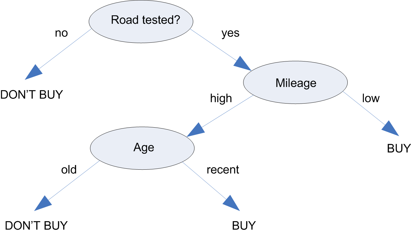
This is a classic case of decision tree algorithm example.
Suppose you have decided to buy a used car, but you are stressing on the requirement that the mileage should be high.
Thus, if initially, you come to know that the mileage is low, you would reject the idea of buying the car, but if the mileage is high, you will go one step further and see how old the car is. If it is recent, you will buy it, if not, you won’t.
Such kind of decision making is done by humans on a regular basis, and the tree shown above that represents the decision-making process is called a predictive model, which predicts a further step on the basis of existing data of previous steps.
The importance of the decision tree algorithm in machine learning is often stressed upon stating this similarity with humans’ decision-making methodology.
With various languages being popular for data science and machine learning, decision tree algorithm in Python is an attractive combination.
The Terminology of a Decision Tree
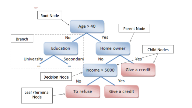
Although it might look like a lot of boxes, for now, pay attention only to the white boxes that make up the terminology of a decision tree and you will understand what is what.
1. Root Node
The root node is the largest (undivided) sample of data at the beginning, which further gets split into two or more homogeneous sets.
While deciding on a root node, the best attribute is often selected to optimize processing; for example, in the above example, it does not make sense to process other decisions if the person is 20 years of age.
2. Branch
A sub-section of the tree is called a branch.
3. Parent Nodes and Child Nodes
Any node split into sub-nodes is a parent node and the split nodes are called child nodes.
4. Decision Node
Any node that splits into sub-nodes can be called a Decision Node. E.g. Splitting of the node ‘utensils’ into the sub-nodes ‘plates’ and ‘bowls’.
In other words, the node that makes the decision that leads to the split is a decision node. Technically, every node that is not a leaf node can be called some sort of a decision node.
5. Leaf Node
The final nodes that do not split further are called Leaf Nodes or Terminal Nodes.
E.g. A batch of students sequentially split according to gender, age, height, and weight will further probably not need splitting, thus becoming a Leaf Node.
6. Splitting
The process of splitting a Node into two sub-nodes is called splitting. It occurs at all nodes except leaf nodes. E.g. Splitting of a group of students according to gender.
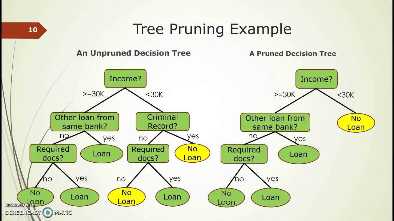
7. Pruning
When we reduce the size of a tree (even literally) by removing any nodes/sub-nodes, it is called pruning. Pruning can be thought of as the opposite of splitting.
Pruning reduces the complexity of the final classifier. This is helpful in improving the accuracy of the prediction by reducing the problem of overfitting in the decision tree algorithm, which we will see later.
Basic Types
We have noted earlier that a decision tree algorithm is a predictive model, i.e., it predicts an output for a new input based on previous data.
Decision tree algorithms are essentially algorithms for the supervised type of machine learning, which means the training data provide to trees is labelled.
The job of a decision tree is to make a series of decisions to come to a final prediction based on data provided.
This final result is achieved in two different ways:
1. Classification
Classification problems are when the predicted values can be categorized into one of the categories as a discrete value.
For example, the categorization of students into male and female is a classification problem and the decision tree can be called a classification tree. Both the previous examples we encountered in this article are examples of classification problems.
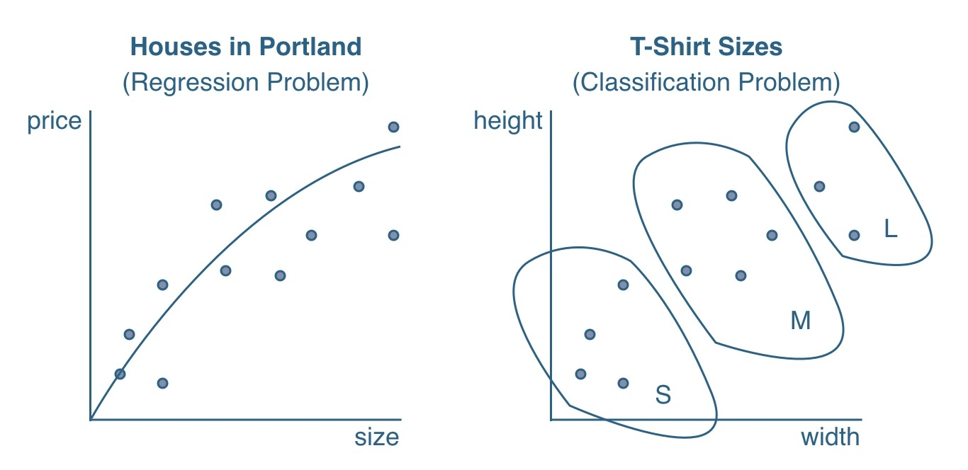
2. Regression
A regression problem is when the predicted output values are not discrete but continuous, such as predicting the price of a house of a given size based on previous data on sizes and corresponding prices.
Thus, the target value now cannot be of yes/no type such as male or female, but a continuous value.
The terminal nodes here obtain value from the training data by taking the mean response of the observations in that region.
The following image shows a decision tree algorithm example with the difference between classification and regression problems that it handles.
Working of a Typical Decision Tree Algorithm in Machine Learning
The following steps are generally followed while setting up a decision tree:
(i) The best attribute is first placed at the Root Node, such as whether a car is in operating condition or not. If it is, only then further splitting will be done based on age, mileage, etc. This simplifies the tree to a large extent. Having the smallest and simplest tree leads to faster and more accurate processing of data.
(ii) Splitting of training data into subsets is done, such as male and female.
(iii) The above steps are repeated until we arrive at a terminal node or a leaf node beyond which subsets cannot or need not be created.
(iv) Typically a decision tree follows the greedy algorithm approach, where it tries to make an optimal choice at every step of splitting, locally. It focuses on the step itself at a time while making a choice, thus the name.
One can use a decision tree algorithm in Python language or R or other supported languages but the overall pseudocode remains similar.
Assumptions
Some basic assumptions are made while working on a decision tree.
(i) The training data given is always as considered the root.
(ii) Although in regression models the output can be a continuous value, the input has to be a discrete value. Thus, if continuous values exist in the training data, the discretization of such values has to be done.
An important question arises while understanding Decision Trees is the basis of the selection of attributes for splitting, which takes us to the topic of attribute selection methods.
Attribute Selection
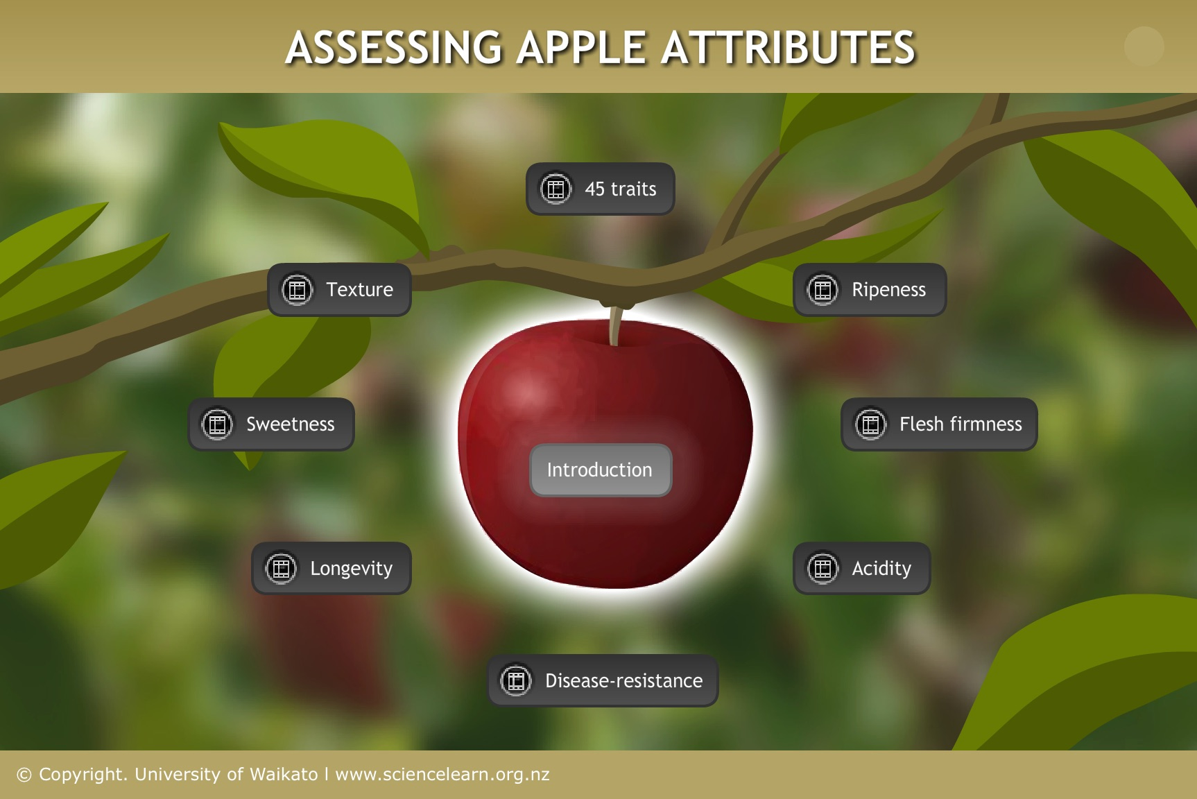
An attribute is a feature of a variable, such as ‘red’ is one of the attributes of the fruit ‘apple’. While splitting data, it is done on the basis of an attribute. For example, fruits can be split on the basis of their colour, or the size, or for specific sciences, there can be many complex attributes like this image.
The selection of attribute is a very important and decisive step in the decision tree algorithm as it decides the complexity and accuracy.
The best attribute is the one which gives the smallest and simplest tree, thus saving time, computing resources, and even cost.
Attribute Selection is a way of ranking attributes among which the one with the higher ranking will be selected as the splitting attribute. The following are the common methods used for the attribute selection process.
1. Information Gain
The goal of selecting an attribute is to select one which can give maximum information about a class. The ‘Information Gain’ method focuses on this logic and tries to select an attribute that maximizes information gain.
But how does information gain work? IG uses a term called entropy.
Entropy means different things in thermodynamics and statistics, and thankfully, the one in statistics is not so complicated as the former.
Entropy is a measure of disorder in a set of data or the measure of uncertainty/impurity. It has a relatively simple equation for itself:

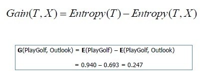
The more the entropy of a case, the lesser the proper information. Let us take a decision tree algorithm example where you want to decide on whether you will play golf or not.
Let’s consider a scenario where you are trying to decide on playing something.
At the first stage when you are only deciding on whether you feel like playing golf, the information is low and entropy is high.
In stage two, you have also considered the factor of weather, which will also aid in deciding whether you will finally go and play.
In this case, the information increased (was gained) in stage 2 and the entropy was decreased. Thus, measuring entropy gives us the measure of entropy loss and helps in the selection of an attribute.
Here’s an informative video that explains information and entropy from the computer science view by taking a relatable decision tree algorithm example:
2. Gini
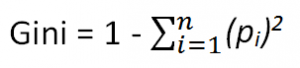
Unlike IG, the Gini index is a measure of impurity of a class or the probability of a variable being classified wrongly when randomly chosen.
It varies between 0 and 1. A value of 0 means no impurity, or that all variables belong to that class, while 1 means all elements are randomly distributed across various classes.
The formula for the same goes like this:
Advantages of Decision Tree Algorithm
(i) It is simple to understand, as well as explain, as it is very similar to human data processing ways.
(ii) Relatively less effort is required from the user for data preparation.
(iii) Decision trees are very flexible in nature, in the sense that they do not need completely comprehensive data like other algorithms. Some missing features are tolerated.
Limitations of Decision Tree Algorithm
(i) The most common and probably the most talked about limitation is overfitting. Overfitting means that the algorithm overlearns things in a way that it treats some noise and fluctuations in the data as learning concepts, thus making errors. Overfitting causes too many tree branches and increased complexity resulting in reduced accuracy.
(ii) The greedy approach of local splitting may produce great local results (minimum impurities at that step) but cannot work optimally on all levels at once. In everyday terms, it is shortsighted.
(iii) With an increase in the size and complexity of data, the size and complexity of the tree also increase, thus reducing accuracy. Decision trees are hence not great for large, complex sets of data.
Wrapping Up
To conclude, the decision tree algorithm in machine learning is a great, simple mechanism and quite valuable in the big data world.
As you read this, somewhere a decision tree algorithm in Python or elsewhere is accurately predicting a life-threatening disease in a patient.
If you are pondering on the idea of learning more about it and exploring the field of machine learning, congratulations! You are having a great idea.
If you are also inspired by the opportunity that Data Science provides, enroll in the Data Science Course & upgrade your career as a Data Scientist.