
The primary job of a data analyst is to make sense out of raw data. Excel has a number of tools to help with this. In this post, we will focus on useful functions towards this purpose. These functions are categorised into different sections like statistical, logical, financial, etc. We will look at a few conditional, summarizing, statistical & logical functions. Let’s dive right in:
Sample Data:
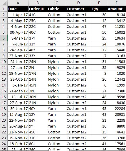
Our sample dataset consists of 212 rows of sale details for textile. We will be using this as an example.
1) Recoding & Frequencies
The if function basically allows you to set up a condition for excel to evaluate. This can be very useful if certain data needs to be recorded. For example, from our dataset, if you need to see the most frequently ordered fabric, there is a statistical function called MODE. But there is a drawback, the function only works on numbers; not on text. If we try that we get a #N/A error. But if we can convert the fabrics to numbers, we can easily get the answer.
To do this, we can use the if function. The basic format (syntax) is:
=IF(logical_test, [value_if_true], [value_if_false])
Using this format, our function would look like this:
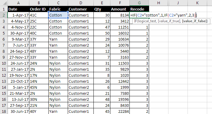
=IF(C2=”cotton”,1, IF(C2=”yarn”,2, 3))
This makes excel check if the value in cell C2 is equal to “cotton”, it will output 1. If not, it will check if is “yarn”. If it is, it will output 2; if not, it can only be “nylon” therefore 3.
Now, we can run a lot of functions that work only on numerical values; for instance, the MODE function. It is a simple function to check for the most frequently occurring item. If you run the MODE function on the recoded column, the answer would be 1. This shows that cotton is the most frequently ordered fabric.
2) Conditional Addition
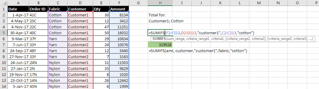
Almost everyone knows how to add up numbers, but you can also sum up numbers based on specific criteria. For example, we need a total amount that has been paid by customer1 for cotton. This can be done using the SUMIFS function. The input would look like this:
=SUMIFS(amt range, customer range,“customer1”, fabric range, “cotton”)
This returns a total of 3,19,028.
3) Criteria based counts
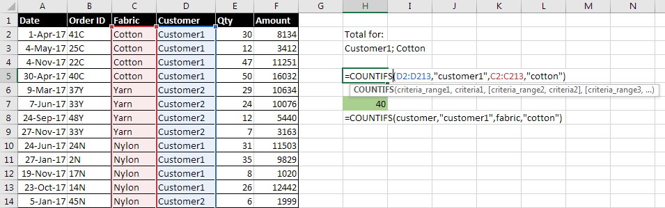
We can also get a count for the same criteria. The COUNTIFS function does not have to have a separate range on which to calculate on, as it simply counts whatever values are present. In the case of SUMIFS, it is not possible to add up text per se. Therefore, there you need to specify a separate range with all the numbers to add up.
=COUNTIFS(customer range,“customer1”,fabric range, “cotton”)
This returns a count of 40 orders.
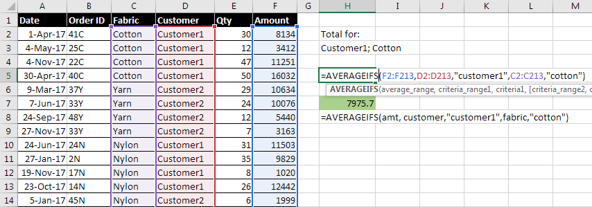
4) Selective Averages
Similarly, we can get an average for the same criteria. The syntax stays the same as =SUMIFS; as the average cannot be calculated on text values. Therefore, a separate range with the numbers has to be specified, based on which it will pick up only the numbers that are in the same row as the criteria; and perform calculations on just those.
=AVERAGEIFS(amt range, customer range,“customer1”,fabric range,“cotton”)
This results in 7975.7 as the average of given criteria.
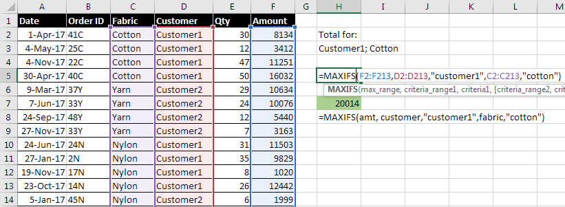
5) Maximum within a condition
The MAXIFS function can be used to return the highest value within a given criterion. Again, this function will depend on number values.
=MAXIFS(amt range, customer range,“customer1”, fabric range, “cotton”)
This results in 20,014 as the highest value.
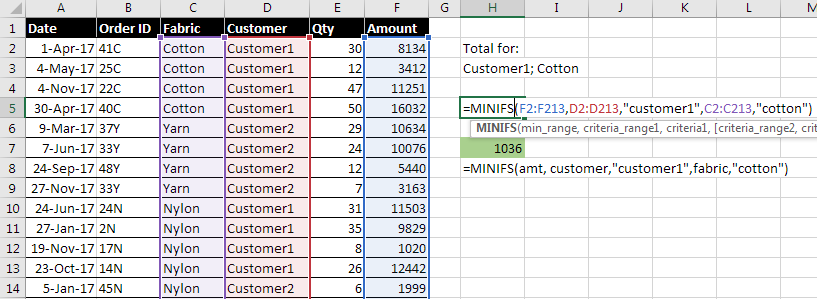
6) Minimum within a condition
The MINIFS function can be used to return the lowest value within a given criterion.
=MINIFS(amt, customer,“customer1”,fabric,“cotton”)
This results in 1,036 as the lowest transaction amount in our dataset:
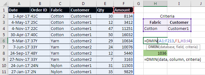
7) Lowest values from Database
Another, lesser known way to perform conditional calculations, is by using Database Functions. Using the same example, the method for calculating the lowest transaction amount in our dataset would be:
=DMIN(data, column to calculate, criteria)
Parameters:
Data – Full dataset, including headers
Column – The index number or label of the column to calculate on
Criteria – A smaller table listing out all the criteria with corresponding labels to base calculations on
8) Highest values from Database
For this, we can use the function DMAX with the following syntax:
=DMAX(data, column to calculate, criteria)
Now, the question of usefulness arises. If the same things can be done with the MINIFS & MAXIFS functions, why bother doing the database versions to get the same result? The advantage of using database functions is that you can list out multiple criteria quickly without writing long and complicated formulas.
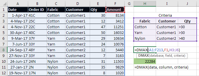
So, let’s say we need to find the maximum amount that fits the following criteria:
|
Maximum in: |
||
|
Fabric |
Customer |
Qty |
| Cotton | Customer1 | >30 |
| Yarn | Customer1 | >30 |
| Nylon | Customer2 | >40 |
Imagine typing all that into a MAXIFS function!
But with the DMAX function, it is very simple:
=DMAX(data, column to calculate, criteria)
Which outputs 22,284 as the maximum value.
9) N from a Database
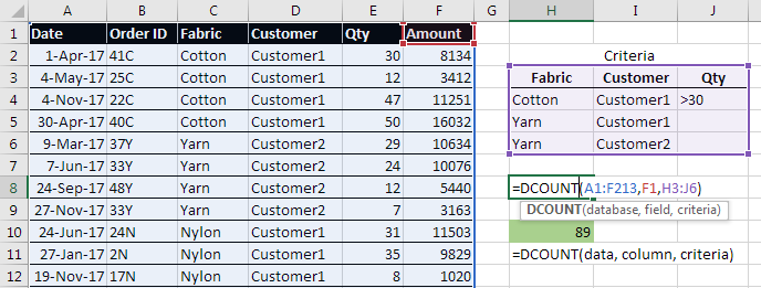
Similarly, we can count all values that fit a set of criteria using the DCOUNT function. The syntax is similar for every database function:
=DCOUNT(data, column to calculate, criteria)
Another trait of database functions is that the layout of your criteria is critical. All the labels in the criteria must match the labels in the dataset. For example, in our dataset, the quantity column is labelled ‘Qty’. If we write ‘Quantity’ in our criteria, Excel will not be able to locate where the column ‘Quantity’ is.
When there are multiple columns of criteria, whatever criteria is put on a single row will mean all of it must be true for evaluation to happen. This is demonstrated in our next set of criteria for counting:
|
Counts of: |
||
|
Fabric |
Customer |
Qty |
| Cotton | Customer1 | >30 |
| Yarn | Customer1 | |
| Yarn | Customer2 | |
Here, the first row of criteria means any order that is Cotton AND is from Customer1 AND is greater than 30 in quantity will be counted.
The second row of criteria means any order that is Yarn AND is from Customer1 will be counted. In the third one only Yarn AND Customer2 will be counted.
This returns a count of 89 orders.
10) Summation from Database
You can also setup criteria like this:
|
Criteria |
|
|
Fabric |
Customer |
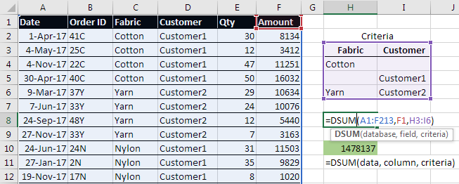
| Cotton | |
| Customer1 | |
| Yarn | Customer2 |
Here, in the first row, we are summing up all the orders for cotton. In the second row, we get a total of all the orders of Customer1. In the third row, we sum up all the yarn orders for Customer2. So, excel reads this as – Cotton OR Customer1 OR Yarn of Customer2. The syntax looks like:
=DSUM(data, column to calculate, criteria)
Any database function will have these quirks. You can also use the DAVERAGE function in a similar way.
11) VLOOKUP
As a data analyst, you may sometimes need to see the details of individual orders. This can be done easily with VLOOKUP. Although a well-known function, it has its own limitations. The foremost being that it can only search in the first column, and then on the right side only. Let’s look at our example. We need to extract the Fabric, Quantity and Amount for a given order number. To do this we can layout a simple table like this:
|
Required Details |
|
| Order ID | |
| Fabric | |
| Quantity |
|
| Amount |
|
The syntax of VLOOKUP is quite simple:
=VLOOKUP(lookup_value, table_array, column_index_num, range)
- First, it needs a value to search with.
- Next, it needs the dataset to search within.
- Once it finds a matching value, it needs to know which corresponding column has the needed data.
- For the last parameter, we will only look at exact matches right now. We do this by putting a zero.
|
Required Details |
||
| Order ID | 25c | |
| Fabric | Cotton | =VLOOKUP(order ID, data, column# containing fabrics,0) |
| Quantity |
12 |
=VLOOKUP(order ID, data, column# containing qty,0) |
| Amount |
3412 |
=VLOOKUP(order ID, data, column# containing amt,0) |
Here, as the Order ID changes, all the other details will be collected for you from the data.
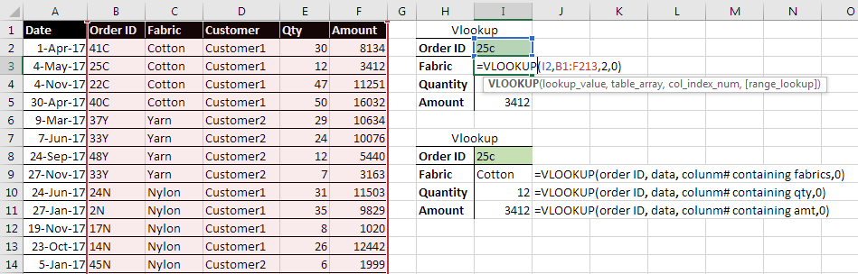
Did you notice, my selection of data starts only from the Order ID column? This done intentionally so that VLOOKUP can search the Order IDs. It can only search in the first column of whatever data is given to it.
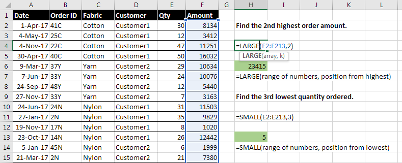
12) Nth value from a dataset
The max and min functions only show the highest and lowest values. But if you want to find out the 2nd highest or 10th lowest, you need to use the LARGE and SMALL functions:
=LARGE(range of numbers, position from highest)
=SMALL(range of numbers, position from lowest)
In our example, we need to find out the 2nd highest order amount & 3rd lowest quantity ordered, respectively. The second parameter is where you specify the required position. So, if you put 1, it will give the maximum / minimum value. If you put 2, it will give you the 2nd highest / lowest value.
13) Standard Deviation
An analysis of data will need some statistical knowledge to have a better understanding of it. The standard deviation is a nifty tool to do so. It is basically a measure of how much the data spreads and deviates from its middle point (Median). It can be calculated on the whole dataset (Population) or just a part of it (Sample). To calculate the standard deviation of the quantities in Excel, we will use the STDEV.P function to calculate on our entire dataset. It needs only a set of numbers; no other parameters needed:
=STDEV.P(numbers)
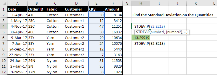
If we had to calculate on a part of our dataset, you can also use the STDEV.S function in a similar way.
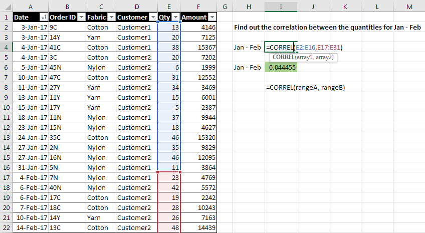
14) Correlation
Correlation is the similarity between 2 sets of values. We can use this to find out how the orders of one month stack up against the orders of another. The only requirement is to have an equal number of values for both the months. In our example, you can see how quantities for January and February correlate:
=CORREL(RANGE1, RANGE2)
15) Subtotals
Lastly, filtering will be a well-worn tool to go through data. Once you use filter out data, running calculations on the filtered data can be done by the SUBTOTAL function. This will ensure all the data that is filtered out stays out. For example, if we compare the SUM function with the SUBTOTAL function, we get vastly different results:
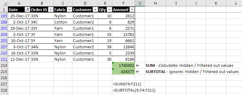
Usually, functions do not consider the visibility of cells. But the Subtotal function will do so. Its syntax is a little different in that first you have to specify what it must do. Then you give it the range of values to calculate on.
=SUBTOTAL(function number, range of values)
The first parameter is a numerical code for the kind of calculation needed. So, to sum, the value is 9. When you type the function in excel, it will give you a list of all the available functions. You just type the number or double-click on it. A quicker way is to use the arrow keys to go down the list and then press tab to select one. The second parameter consists of just the range of numbers.
Thus, Using all these functions, and many more, a data analyst can carry out his/her job extremely well and much more efficiently. If the data analyst had to carry out all these calculations manually, there would be a huge time loss and great changes due to human errors.
These functions help the data analyst to spend more time on building logic, coming up with solutions that help in better and faster decision making, rather than spending time doing these calculations. Excel has many more features and functions that a data analyst can use on a daily basis, but these 15 are a must to know.
If you are also want to build a strong career in Data Science and Analytics, enroll in the Data Science Master Course today.


Can you please provide the xls datasheet so that we can practice hands on ?