Do you want to know how to analyze data in excel?
Are you looking for the best way to analyze data in excel?
Keep Reading!
Microsoft Excel is one of the most widely used tools in any industry. While some enjoy playing with pivotal tables and histograms, others limit themselves to simple pie-charts and conditional formatting.
Some may create an artwork out of the dull monochrome Excel, while others may be satisfied with its data analysis. In this discussion, we will make a deep delving analysis of Microsoft Excel and its utility. We will focus on how to analyze data in Excel Analytics, the various tricks, and techniques for it. The discussion will also explore the various ways to analyze data in Excel.
We will discuss the different features of Excel analytics to know how to analyze data in excel (much of which are unexplored to the mass), functions, and best practices.
Our discussion will include, but not be limited to:
(i) Best Way to Analyze Data in Excel
(ii) How to Analyze Sales Data in Excel
(iii) Analyzing Data Sets with Excel
(iv) Data Segregation with Excel
(v) The Importance of Data Reporting
(vi) How to Analyze Data in Excel
How to Analyze Sales Data in Excel: Make Pivot Table your Best Friend
A pivot tool helps us summarize huge amounts of data. One of the best ways to analyze data in excel, it is mostly used to understand and recognize patterns in the data set.
Recognizing patterns in a small dataset is pretty simple. But the enormity of the datasets often calls for additional efforts to find the patterns. In such cases, a pivot table can be a huge advantage as it takes only a few minutes to summarize groups of data using a pivot table.
A data analysis example can be, you have a dataset consisting of regions and number of sales. You may want to know the number of sales based on the regions, which can be used to determine why a region is lacking and how to possibly improve in that area. Using a pivot table, you can create a report in excel within a few minutes and save it for future analysis.
A Pivot Table allows you to summarize data as averages, sums, or counts in Excel from data that is stored in another Spreadsheet, or table. It is great for quickly building reports because you can sort and visualize the data quickly.
Taking a data analysis example like, you may have put together a spreadsheet, which you can copy, and paste into Excel, or use in Google Docs if you would prefer (just click File > Make a Copy).
The spreadsheet contains data with a mock company’s customer purchase information. Since companies purchase at different dates, a pivot table will help us to consolidate this data to allow us to see total buys per company, as well as to compare purchases across companies, for quick analysis.
The Pivot table allows you to take a table with a lot of data in it and rearrange the table so that you only look at only what matters to you.
- a) Whether you are using a Mac or a PC, you can select the whole dataset that you want to look at and select: “Data” -> “Pivot Table”. When you hit that, a new tab should be opened with a table.
Data Set
- b) Once you have your table in front of you, you can drag and drop the Column Labels, Row Labels, and Report Filter
- Column Labels go across the top row of your table (for example Date, Month, Company Name)
- Row Labels go across the left-hand side of your table [for example Date, Month, Company Name (same as with column labels, it depends on how you would prefer to look at the data, vertically or horizontally)]
- The Values section is where you put the data you would like calculated (for example Purchases, Revenue)
- Report Filter helps you refine your results. Add anything you would like to Filter by (for example you want to look at Lead Referral Sources, but exclude Google and Direct)
Pivot tables are a great way to manage the data from your reports. You can copy and paste the data into your own Excel file, or create a copy in Google Apps (File > Make a Copy).

How to Analyze Data in Excel: Analyzing Data Sets with Excel
To know how to analyze data in excel, you can instantly create different types of charts, including line and column charts, or add miniature graphs. You can also apply a table style, create PivotTables, quickly insert totals, and apply conditional formatting. Analyzing large data sets with Excel makes work easier if you follow a few simple rules:
- Select the cells that contain the data you want to analyze.
- Click the Quick Analysis button image button that appears to the bottom right of your selected data (or press CRTL + Q).
- Selected data with Quick Analysis Lens button visible
- In the Quick Analysis gallery, select a tab you want. For example, choose Charts to see your data in a chart.
- Pick an option, or just point to each one to see a preview.
- You might notice that the options you can choose are not always the same. That is often because the options change based on the type of data you have selected in your workbook.
To understand the best way to analyze data in excel, you might want to know which analysis option is suitable for you. Here we offer you a basic overview of some of the best options to choose from.
- Formatting: Formatting lets you highlight parts of your data by adding things like data bars and colors. This lets you quickly see high and low values, among other things.
- Charts: Charts Excel recommends different charts, based on the type of data you have selected. If you do not see the chart you want, click More Charts.
- Totals: Totals let you calculate the numbers in columns and rows. For example, Running Total inserts a total that grows as you add items to your data. Click the little black arrows on the right and left to see additional options.
- Tables: Tables make it easy to filter and sort your data. If you do not see the table style you want, click More.
- Sparklines: Sparklines are like tiny graphs that you can show alongside your data. They provide a quick way to see trends.

Ways to Analyze Data in Excel: Tips and Tricks
It is fun to analyze data in MS Excel if you play it right. Here, we offer some quick hacks so that you know how to analyze data in excel.
-
How to Analyze Data in Excel: Data Cleaning
Data Cleaning, one of the very basic excel functions, becomes simpler with a few tips and tricks. You may learn how to use a native Excel feature and how to accomplish the same goal with Power Query. Power Query is a built-in feature in Excel 2016 and an Add-in for Excel 2010/2013. It helps you to extract, transform, and load your data with just a few clicks.
1. Change the format of numbers from text to numeric
Sometimes when you import data from an external source other than Excel, numbers are imported as text. Excel will alert you by showing a green tooltip in the top-left corner of the cell.
Depending on the number of values in the range, you can quickly convert the values to numbers by clicking on ‘Convert to a number’ within the tooltip options.
However, if you have more than 1000 values, you will have to wait a couple of seconds while Excel finishes the conversion.
You may also convert the values to number format is to use Text-to-Columns using the following steps:
- Select the range with the values to be converted.
- Go to Data > Text to Columns.
- Select Delimited and click Next.
- Uncheck all the checkboxes for delimiters (see below) and click Next.
- Text-Columns-Checkboxes
2. Select General and click on Finish
When you have lots of numbers to convert this tip will be much faster than waiting for all the numbers to be converted. In Power Query, you just have to right-click on the column header of the column you want to convert.
- Then go to Change Type.
- Then select the type of number you want (such as Decimal or Whole Number)
- Power-Query-Data-Type
How to Analyze Data in Excel: Data Analysis
Data Analysis is simpler and faster with Excel analytics. Here, we offer some tips for work:
- Create auto expandable ranges with Excel tables: One of the most underused features of MS Excel is Excel Tables. Excel Tables have wonderful properties that allow you to work more efficiently. Some of these features include:
- Formula Auto Fill: Once you enter a formula in a table it will be automatically be copied to the rest of the table.
- Auto Expansion: New items typed below or at the right of the table become part of the table.
- Visible headers: Regardless of your position within the table, your headers will always be visible.
- Automatic Total Row: To calculate the total of a row, you just have to select the desired formula.
- Use Excel Tables as part of a formula: Like in dropdown lists, if you have a formula that depends on a Table, when you add new items to the Table, the reference in the formula will be automatically updated.
- Use Excel Tables as a source for a chart: Charts will be updated automatically as well if you use an Excel Table as a source. As you can see, Excel Tables allow you to create data sources that do not have to be updated when new data is included.
How to Analyze Data in Excel: Data Visualization
Quickly visualize trends with sparklines: Sparklines are a visualization feature of MS Excel that allows you to quickly visualize the overall trend of a set of values. Sparklines are mini-graphs located inside of cells. You may want to visualize the overall trend of monthly sales by a group of salesmen.
To create the sparklines, follow these steps below:
- Select the range that contains the data that you will plot (This step is recommended but not required, you can select the data range later).
- Go to Insert > Sparklines > Select the type of sparkline you want (Line, Column, or Win/Loss). For this specific example, I will choose Lines.
- Click on the range selection button Select Range Excel Button to browse for the location of the sparklines, press Enter and click OK. Make sure you select a location that is proportional to the data source. For example, if the data source range contains 6 rows then the location of the sparkline must contain 6 rows.
To format the sparkline you may try the following:
To change the colour of markers:
- Click on any cell within the sparkline to show the Sparkline Tools menu.
- In the Sparkline tools menu, go to Marker Color and change the colour for the specific markers you want.
For example High points on the green, Low points on red, and the remaining in blue.
To change the width of the lines:
- Click on any cell within the sparkline to show the Sparkline Tools menu.
- In the Sparkline tools contextual menu, go to Sparkline Color > Weight and change the width of the line as you desire.
Save Time with Quick Analysis: One of the major improvements introduced back in Excel 2013 was the Quick Analysis feature. This feature allows you to quickly create graphs, sparklines, PivotTables, PivotCharts, and summary functions by just clicking on a button.
When you select data in Excel 2013 or later, you will see the Quick Analysis button Quick Analysis Excel Button in the bottom-right corner of the range selected. If you click on the Quick Analysis button you will see the following options:
- Formatting
- Charts
- Totals
- Tables
- Sparklines
When you click on any of the options, Excel will show a preview of the possible results you could obtain given the data you selected.
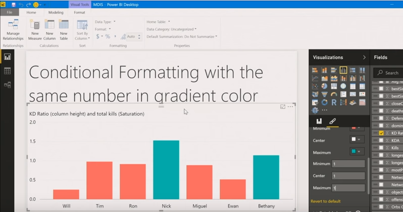
- If you click on the Quick Analysis button and go to charts, you could quickly create the graph below just by clicking a button.
- If you go to Totals, you can quickly insert a row with the average for each column:
- If you click on Sparklines, you can quickly insert Sparklines:
- As you can see, the Quick Analysis feature really allows you to quickly perform different visualizations and analysis with almost no effort.
How to Analyze Data in Excel: Data reporting
Data reporting in Excel analytics requires more than just accounting skills, it also requires a thorough knowledge of excel functionalities and the ability to add beauty to your report.
- Turn Auto Refresh off before editing the Excel workbook. This will stop the table from refreshing when you are making changes on the worksheet. To do this, click on the Refresh icon at the bottom of the Excel Report Designer Task Pane and then select “Switch auto-refresh off”.
- When adding a new row to the layout, select a cell in the table area below where you want to insert the new row. Then right-click and from the context menu select Insert > Table Rows Above.
- When deleting columns or rows make sure you use the Table Delete functions similar to the Insert functions above. To remove a column or row, select a cell in the table area of the row or column you want to remove. Then right-click and from the context menu select Delete and then either Table Columns or Table Rows.
- Remove unneeded rows or columns from the table. Having fewer cells in the layout makes it easier for the table to refresh, so removing any unneeded ones will improve performance.

Excel has several other uses that may not have been covered here. Play around with visualize complex data or organize disparate numbers, to discover the infinite variety of functions in Excel analytics. Strong knowledge of excel is a boon if you are looking forward to a career in data analytics.
This was all about how to analyze data in excel, how to analyze sales data in excel along with a few data analysis example.
Hopefully, you must have understood the best way to analyze data in excel.
We offer one of the best-known courses in Data Analytics Using Excel Course. The course enables you to learn tools such as Advanced Excel, PowerBI, and SQL. The live projects and intensive training program also empower you to come up with solutions for real-life problems.