Types of Linear Programming Problems: Concepts & Solutions

Linear programming problems consist of a linear function to be maximized or minimized. Linear Programming is a method of performing optimization that is used to find the best outcome in a mathematical model. In linear programming, the objective function (the linear function representing the quantities to be maximized or minimized) and the constraints (the system of equalities or inequalities describing the restrictions on the decision variables) are represented by the linear relationships.

Watch: How to Solve a Linear Programming Problem Using a Graphical Method!

Linear Programming Problems Terminologies

The following are the terminologies that you must be familiar with before you start with linear programming problems:

Objective Function

It is defined as some numerical value that should be maximized or minimized. For example, if you are involved in some business, then your primary goal is to maximize profits and reduce loss.

Constraints

The constraints are defined as the limitations of the decision variables. For example, if you are involved in some business, then the budget, number of workers, production capacity, space, etc. are the limitations or restrictions.

Decision Variables

Decision variables are the variables that decide the output. For example, if you are a farmer who wants to grow wheat and barley, then calculating the total area for growing wheat and barley are the decision variables.

Non-negativity Restriction

Non-negativity restriction means that the values for decision variables should be greater than or equal to 0.

How to Define a Linear Programming Problem?

For a problem to be defined as a linear programming problem, all the decision variables, objective function, and constraints must be linear functions. The following are the steps for defining a problem as a linear programming problem:

(1) Identify the number of decision variables
(2) Identify the constraints on the decision variables
(3) Write the objective function as a linear equation
(4) Explicitly state the non-negativity restriction
(5) Linear Programming Problems

A linear programming problem deals with a linear function to be maximized or minimized subject to certain constraints in the form of linear equations or inequalities.

In this section, we will learn how to formulate a linear programming problem and the different methods used to solve them.

Problem Statement:

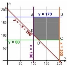
A calculator company manufactures two types of calculator: a handheld calculator and a scientific calculator. Statistical data projects that there is an expected demand of at least 100 scientific and 80 handheld calculators each day. Since the company has certain limitations on the production capacity, the company can only manufacture 200 scientific and 170 handheld calculators per day. The company has received a contract to deliver a minimum of 200 calculators per day. If there is a loss of 2INR on each scientific calculator that you sold and a profit of 5INR on each handheld calculator, then how many calculators of each type the company should manufacture daily to maximize the net profit?

Solution:

To solve this problem, let’s first formulate it properly by following the steps stated above.

Step 1: Identify the number of decision variables. In this problem, since we have to calculate how many calculators of each type should be manufactured daily to maximize the net profit, the number of scientific and handheld calculators each are our decision variables.

X = number of scientific calculators manufactured

Y = number of handheld calculators manufactured

Hence, we have two decision variables in this problem.

Step 2: Identify the constraints on the decision variables.

The lower bound, as mentioned in the problem (there is an expected demand of at least 100 scientific and 80 handheld calculators each day) are as follows.

Hence,

X >= 100

Y >= 80

The upper bound owing to the limitations mentioned the problem statement (the company can only manufacture 200 scientific and 170 handheld calculators per day) are as follows:

Hence,

X<=200

Y<=170

In the problem statement, we can also see that there is a joint constraint on the values of X and Y due to the minimum order on a shipping consignment that can be written as:

X + Y >= 200

Step 3: Write the objective function in the form of a linear equation. In this problem, it is clearly stated that we have to optimize the net profit. As stated in the problem(If there is a loss of 2INR on each scientific calculator that you sold and a profit of 5INR on each handheld calculator), the net profit function can be written as:

Profit (P) = -2X + 5Y

Step 4: Explicitly state the non-negativity restriction. Since the calculator company cannot manufacture a negative number of calculators, there is no non-negativity restriction.

Hence,

X ≥ 0

Y ≥ 0

Since we have formulated the problem, let’s convert the problem into a mathematical form to solve it further.

Maximization of P = -2X + 5Y, that is subject to:

100 ≤ X ≤ 200

80 ≤ Y ≤ 170

X + Y ≥ 200

Graphical Method of Solving a Linear programming Problem

The graphical method solves the problem by finding the highest or lowest point of intersection between the objective function line and the feasible region on a graph.

This method solves the problem statement by breaking it into the following steps:

Step 1 to Step 4 is the same as mentioned in formulating a linear programming problem.

Step 5: Plot the constraints on the graph. Let’s plot all the constraints defined in step 2 on a graph in a similar manner as we plot an equation.

To plot the constraint mentioned in step2 on a graph, you must convert the inequality into an equation:

X + Y = 200

Mark the coordinated on the graph and draw a straight line across the coordinates.

Step 6: Highlight the feasible region on the graph. After plotting the coordinates on the graph, shade the area that is outside the constraint limits (which is not possible). The highlighted feasible area will look like this:

Step 7: Find the coordinates of the optimum point. To find the coordinates of the optimum point, we will solve the simultaneous pair of linear equations by taking some random values.

P = -2X + 5Y

Corner Points

Equation, P = -2X + 5Y

A (100, 170)

P = 650

B (200, 170)

P = 450

C (200, 80)

P = 0

D (120, 80)

P = 160

E (100, 100)

P = 300

These corner points coordinates are obtained by drawing two perpendicular lines from the point onto the coordinate axes.

Step 8: Find the optimum point.

The above table shows that the maximum value of P is 650 that is obtained at (X, Y) = A (100, 170).

Solve Linear Program Using R

To solve a linear programming problem using R, you must be familiar with the lp_solve package. This package contains several functions for solving linear programming problems and getting significant statistical analysis. Let’s understand this method with an example.

Example:  A manufacturing company sells two products that are A and B at 25$ and 20$ respectively. The company has only 1800 resource units available every day. Product A requires 20 resource units while Product B requires 12 resource units and both the products require a  production time of 4 minutes. The total available working hours available in a day are 8. What should be the production quantity for each of the products to maximize profits.

Solution: The objective function in the above problem is

Max(Sales) = Max(25A + 20B)

Where,

A is the units of Product A produced

B is the units of Product B produced

A and B are also called decision variables

We have two constraints in the problem that are resource and time.

20A + 12B <= 1800 (Resource Constraint)

4A + 4B <= 8*60 (Time constraint)

Let’s take a look at the code part:

install.packages(“lpSolve”)

## Load the package lpsolve

library(lpSolve)

## Set the coefficients of the decision variables

objective.in  <- c(25, 20)

## Create constraint martix

const.mat <- matrix(c(20,  12, 4, 4), nrow=2, byrow=TRUE)

## define constraints

time_constraint <- (8*60)

resource_constraint <- 1800

## RHS for the constraints

const.rhs <- c(resource_constraint, time_constraint)

## Constraints direction

const.dir  <- c(“<=”, “<=”)

## Find the optimal solution

optimum <-  lp(direction=”max”,  objective.in, const.mat, const.dir,  const.rhs)

## Display the optimum values for A and B

optimum$solution

The output of the above program is:

## [1] 45 75

## Check the value of objective function at optimal point

optimum$objval

## [1] 2625

Conclusion: It is evident from the above output that the company should produce 45 units of Product A and 75 units of Product B to get sales of $2625, which is the maximum sales that the company can get given the constraints.

Linear Programming Problem Statements and Solutions

Problem Statement:

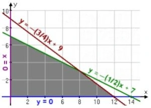
You are an IT organization that wants to equip some new cabinets into your office. You contacted a furniture company, and they informed you that Cabinet X costs $10 per unit, requires 6 square feet of floor space, and holds eight cubic feet of files. The cost of cabinet Y is $20 per unit, requires eight square feet of floor space, and holds twelve cubic feet of files. You have space only for 72 square feet of cabinets and a budget of $140 to make this purchase. How many of which model you should buy to maximize storage volume?

Solution:

To solve this problem, let’s first formulate it properly by following the steps stated above.

Step 1: Identify the number of decision variables. In this problem, since we have to calculate how many of which model we should buy to maximize storage volume, the number of cabinets X and Y are our decision variables.

X = number of model X cabinets purchased

Y = number of model Y cabinets purchased

Hence, we have two decision variables in this problem.

Step 2: Identify the constraints on the decision variables. Costs and space are the two constraints in this problem.

Cost = 10X + 20Y < 140, or Y < –( 1/2 )X + 7

Space = 6X + 8Y < 72, or Y < –( 3/4 )X + 9

Step 3: Write the objective function in the form of a linear equation. In this problem, it is clearly stated that we have to optimize the volume that can be written as:

Volume (V) = 8X + 12Y

Step 4: Explicitly state the non-negativity restriction. Naturally,

X ≥ 0

Y ≥ 0

Since we have formulated the problem, let’s convert the problem into a mathematical form to solve it further.

Step 5: Highlight the feasible region on the graph. After plotting the coordinates on the graph, shade the area that is outside the constraint limits (which is not feasible). The highlighted feasible area will look like this:

Step 6: Find the coordinates of the optimum point. To find the coordinates of the optimum point, we will solve the simultaneous pair of linear equations by taking some random values.

V = 8X + 12Y

Corner Points

Equation, V = 8X + 12Y

A (8, 3)

P = 100

B (0, 7)

P = 84

C (12, 0)

P = 96

These corner points coordinates are obtained by drawing two perpendicular lines from the point onto the coordinate axes.

Step 7: Find the optimum point.

The above table shows that the maximum value of V is 100 that is obtained at (X, Y) = A (8, 3).

Problem Statement:

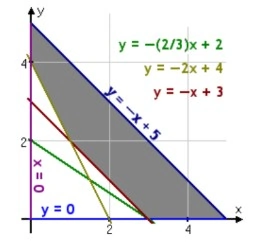
Imagine that you are a lab technician, and your job is to feed rabbits daily. Their daily diet contains a minimum of 24 grams (g) of fat, 36 g of carbohydrates, and 4 g of protein. You can feed only 5 ounces of food per day. It is suitable as per the budget that your order two food products and blend them to obtain an optimal mix. Food X consists of 8 g of fat, 12 g of carbohydrates, and 2 g of protein per ounce, and costs $0.20 per ounce. Food Y includes 12 g of fat, 12 g of carbs, and 1 g of protein per ounce, at the cost of $0.30 per ounce. What is the optimal blend?

Solution:

To solve this problem, let’s first formulate it properly by following the steps stated above.

Step 1: Identify the number of decision variables. In this problem, since we have to calculate the number of ounces of each food required for the optimal daily blend, the number of ounces of Food X and Food Y are our decision variables.

X = number of ounces of Food X

Y = number of ounces of Food Y

Hence, we have two decision variables in this problem.

Step 2: Identify the constraints on the decision variables. The grams of fat, carbohydrates, and protein per ounce are the three constraints in this problem.

Fat = 8X + 12Y > 24

Carbohydrates = 12X + 12Y > 36

Protein = 2X + 1Y >  4

In the problem statement, we can also see that there is a joint constraint on the values of X and Y because the maximum weight of the food is five ounces. Hence,

X + Y <=5

Step 3: Write the objective function in the form of a linear equation. In this problem, it is clearly stated that we have to optimize the cost for the minimum value.

Cost relation, C = 0.2X + 0.3Y

Step 4: Explicitly state the non-negativity restriction. Since, you cannot use negative amounts of either food,

Hence,

X ≥ 0

Y ≥ 0

Since we have formulated the problem, let’s convert the problem into a mathematical form to solve it further.

Step 5: Highlight the feasible region on the graph. After plotting the coordinates on the graph, shade the area that is outside the constraint limits (which is not feasible). The highlighted feasible area will look like this:

Step 6: Find the coordinates of the optimum point. To find the coordinates of the optimum point, we will solve the simultaneous pair of linear equations by taking some random values.

C = 0.2X + 0.3Y

Corner Points

Equation, C = 0.2X + 0.3Y

A (0,4)

C = 1.2

B (0, 5)

C = 1.5

C (3, 0)

C = 0.6

D (5,0 )

C = 1.0

E (1,2)

C = 0.8

These corner points coordinates are obtained by drawing two perpendicular lines from the point onto the coordinate axes.

Step 7: Find the optimum point.

The above table shows that the minimum value of cost = 0.6 and is obtained at (X, Y) = A (3, 0). Hence, you should get a minimum cost of 60 cents per daily serving using 3 ounces of Food X only.

Applications of Linear Programming Problems

Linear programming is used to find optimal solutions for operations research. Linear programming requires the creation of inequalities and then graphing those to solve problems.

Here’s a list of areas where linear programming is used.

Marketing Management

Linear programming allows marketers to analyze the audience coverage of advertising based on constraints such as available media, advertising budge, etc. Linear programming also helps the salespersons (field agents) to determine the shortest route for their destination. A logistic head can easily find the optimal distribution schedule for transporting the product from different warehouses to various market locations in such a manner that the total transport cost is the minimum.

Financial Management

Linear programming helps the financial firms, mutual fund firms, and banks to select the investment portfolio of shares, bonds, etc. in such a manner that the return on investment is maximized.

Inventory Management

Linear programming also helps the inventory firms in the better management of raw materials and finished products. They can find the optimal solution to minimize the inven­tory cost based on space and demand as constraints.

Human Resource Management

Linear programming allows the recruiting manager to solve the problems related to recruitment, selection, training, and deployment of the workforce to different departments of the firm. Linear programming can be used to determine the minimum number of employees required in various shifts to meet the production schedule within a schedule.

Food and Agriculture Management

Linear programming helps farmers to determine which crops to grow, in what quantity the particular crops should be produced to increase their revenue.

Are you interested in Data Science? The demand for data science is huge and expected to grow exponentially. Enroll in Digital Vidya’s Data Science Course to create a strong foundation in Data Science & build a successful career as a Data Scientist. We hope that you find this blog helps you to find answers to specific queries related to linear programming problems. We wish you success and good luck!