Complete Guide to Naive Bayes Classifier

A classifier, in machine learning, is a model or algorithm used to differentiate between objects based on specific features. Naive Bayes Classifiers come under this family of classifiers (probabilistic classifiers to be exact). The naive Bayes classifier is based on the application of Bayes’ theorem with strong (hence the word naive) independence assumptions between the features.

Naive Bayes Classifiers are not a single algorithm, but rather a family of machine learning algorithms that have a common similarity in that every pair of features that are being classified is independent of each other.

You can watch this video for a deeper understanding of naive Bayes Classifiers: Naive Bayes classifier: A friendly approach.

Naive Bayes Classifiers are used in machine learning because they prove to be powerful algorithms for predictive modeling. Why is predictive analysis important?

As data piles up, we have ourselves a genuine gold rush. But data isn’t the gold. I repeat, data in its raw form is boring crud. The gold is what’s discovered therein.

How Naive Bayes Classifier Works

The following Naive Bayes Classifier example will give you an understanding of how Naive Bayes Classifier works.

Consider the above image. The objects in the image can be classified into green or red. Our job is going to be to classify new objects that are introduced into the mix, into green or red, based on the existing information.

Taking probability into consideration, since there are twice as many green objects as red, the probability of a new object (that is not yet observed) that is added being green is twice as the chances of it being red in color. This is known as the prior probability in Bayesian analysis.

Prior probabilities are calculated based on previous experience or information, which in our example is the set of green and red objects. This probability is used to predict outcomes before they happen.

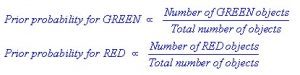
We can formulate this probability as:

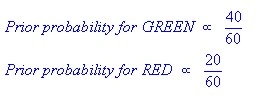
Our example has a total of 60 objects of which 40 are GREEN and 20 are RED. The prior probabilities for class members will be:

With the prior probability defined, we can now predict the outcome of a new object that is added. Consider a new object that is introduced, denoted in white below:

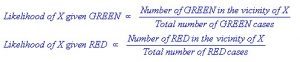
The next observation we make is that the objects are well clustered. We assume that the more green (or red) objects that are clustered around an area ‘X’, the more likely it is for a new object that is introduced in that area to be of that colour.

The white object is circled to make that assumption or likelihood more prominent. We then calculate the number of points within the circle that belong to specific class labels. The expression becomes:

And for our example:

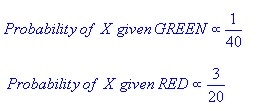
At this point, our prior probabilities indicate the object is likely green (since there are twice as more green objects), but the likelihood indicates the object is more probably red in color, as there are more red objects in the defined vicinity around the new white object.

The Bayesian analysis, the classification is finally deduced by combining the two sources of information: prior probability and likelihood, to form a posterior probability with the help of Bayes’ rule.

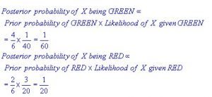
As per the result of the posterior probability, we classify the object as red, since it has a larger posterior probability.

Naive Bayes Classifiers can get more complex than the above Naive Bayes classifier example, depending on the number of variables present.

Consider the below Naive Bayes classifier example for a better understanding of how the algorithm (or formula) is applied and a further understanding of how Naive Bayes classifier works.

The Bayes Theorem is defined as follows:

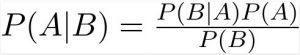
We use Bayes Theorem to find the probability of ‘A’ happening, having known that ‘B’ has occurred. A is called the hypothesis and B is called the evidence. We assume that the features/predictors are independent, which means that one feature does not affect the other (why it is called naive).

Consider the following chart of data:

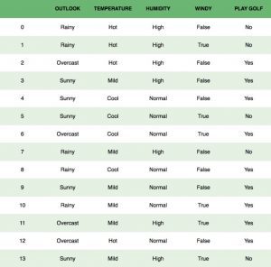
We are trying to classify if a particular day is suitable for playing golf, being given the features of the day. Each column represents a feature, and each row represents individual entries.

If we consider the first row (0), we see that the outlook is rainy, the temperature is hot, and the humidity is high, and hence deduce it is not a good day to play golf. We also assume that each feature is independent, that is the outlook does not impact the temperature, which does not impact any other feature, etc.

The second assumption we make is that all features have an equal effect on the outcome. Which means, just one particular feature cannot outweigh the decision, or have more importance on the outcome.

The Bayes Theorem for this example is written as:

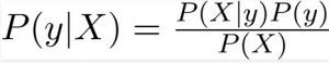
Here, Y is the class variable (whether to play golf or no) and X represents the features or predictors.

X is defined as,

Where x1, x2, etc represent features. When we substitute x for numerous features and expand the formula, we get:

We can now derive values for each by substituting values from the dataset in the following equation:

The denominator for every entry remains constant. Therefore, the equation can be written as:

In our scenario, the class variable Y has just 2 outcomes, yes or no. In cases of higher variations, we need to define Y with maximum probability. The equation becomes:

These examples should give you a good idea of how Naive Bayes classifier works.

Types of Naive Bayes Classifiers

1. Multinomial Naive Bayes

Multinomial Naive Bayes classifier is predominantly used for the document classification problem, to determine if a document belongs to the category of technology, sports, politics, etc. The features that are used in this classifier are words and the frequency of their occurrence in the document.

2. Bernoulli Naive Bayes

The Bernoulli Naive Bayes classifier is similar to the multinomial naive Bayes classifier, but the features/predictors are boolean variables. The features used to predict the class variable only take up values yes or no.

3. Gaussian Naive Bayes

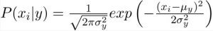
When features/predictors are not discrete and take up a continuous value, it is assumed that the values are sampled from a gaussian distribution. This graph depicts the values:

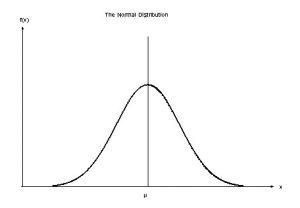
The conditional probability expression for Gaussian Naive Bayes classifiers changes to:

Applications of Naive Bayes Algorithms

Here’s an application of Gaussian Naive Bayes classifier using Scikit-learn.

# load the iris dataset
from sklearn.datasets import load_iris
iris = load_iris()

# store the feature matrix (X) and response vector (y)
X = iris.data
y = iris.target

# splitting X and y into training and testing sets
from sklearn.model_selection import train_test_split
X_train, X_test, y_train, y_test = train_test_split(X, y, test_size=0.4, random_state=1)

# training the model on training set
from sklearn.naive_bayes import GaussianNB
gnb = GaussianNB()
gnb.fit(X_train, y_train)

# making predictions on the testing set
y_pred = gnb.predict(X_test)

# comparing actual response values (y_test) with predicted response values (y_pred)
from sklearn import metrics
print("Gaussian Naive Bayes model accuracy(in %):", metrics.accuracy_score(y_test, y_pred)*100)

The Output would look like:

Gaussian Naive Bayes model accuracy(in %): 95.0

Building a Naive Bayes Classifier in Python

We will build a predictor to predict the species of a flower based on the given measurements using the Iris Flower Species Dataset.

This is a multiclass classification problem. 150 observations are made with 4 input variables and 1 output variable, which are:

• Sepal length in cm
• Sepal width in cm
• Petal length in cm
• Petal width in cm
• Class

Here is a sample of the first 5 rows:

5.1,3.5,1.4,0.2,Iris-setosa
4.9,3.0,1.4,0.2,Iris-setosa
4.7,3.2,1.3,0.2,Iris-setosa
4.6,3.1,1.5,0.2,Iris-setosa
5.0,3.6,1.4,0.2,Iris-setosa

Execution of Naive Bayes Classifier Tutorial for Python

This Naive Bayes classifier tutorial for Python will be executed in 5 steps:

• Class Separation
• Dataset Summarization
• Data Summary by Class
• Gaussian Probability Density Function
• Class Probabilities

Step 1 – Class Separation

The first step is to separate the training data by class. We can use the separate_by_class() function.

# Split the dataset by class values, returns a dictionary
def separate_by_class(dataset):
separated = dict()
for i in range(len(dataset)):
vector = dataset[i]
class_value = vector[-1]
if (class_value not in separated):
separated[class_value] = list()
separated[class_value].append(vector)
return separated

We use the following dataset (sample is below) to test the function:

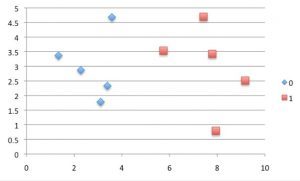
A scatter diagram of the data:

Running the function on the data set:

# Example of separating data by class value

# Split the dataset by class values, returns a dictionary
def separate_by_class(dataset):
separated = dict()
for i in range(len(dataset)):
vector = dataset[i]
class_value = vector[-1]
if (class_value not in separated):
separated[class_value] = list()
separated[class_value].append(vector)
return separated

# Test separating data by class
dataset = [[3.393533211,2.331273381,0],
[3.110073483,1.781539638,0],
[1.343808831,3.368360954,0],
[3.582294042,4.67917911,0],
[2.280362439,2.866990263,0],
[7.423436942,4.696522875,1],
[5.745051997,3.533989803,1],
[9.172168622,2.511101045,1],
[7.792783481,3.424088941,1],
[7.939820817,0.791637231,1]]
separated = separate_by_class(dataset)
for label in separated:
print(label)
for row in separated[label]:
print(row)

And the output is:

0
[3.393533211, 2.331273381, 0]
[3.110073483, 1.781539638, 0]
[1.343808831, 3.368360954, 0]
[3.582294042, 4.67917911, 0]
[2.280362439, 2.866990263, 0]
1
[7.423436942, 4.696522875, 1]
[5.745051997, 3.533989803, 1]
[9.172168622, 2.511101045, 1]
[7.792783481, 3.424088941, 1]
[7.939820817, 0.791637231, 1]

Step 2 – Dataset Summarization

In the second step of this Naive Bayes classifier tutorial, we need to derive 2 statistics from this data set: the mean and the standard deviation.

The mean can be calculated using the formula:

mean = sum(x)/n * count(x)
x – list of values or a column we are checking

We use the below function to calculate mean:

# Calculate the mean of a list of numbers
def mean(numbers):
return sum(numbers)/float(len(numbers))

The formula to calculate the standard deviation is:
standard deviation = sqrt((sum i to N (x_i – mean(x))^2) / N-1

The below function can be used to execute this:

from math import sqrt

# Calculate the standard deviation of a list of numbers
def stdev(numbers):
avg = mean(numbers)
variance = sum([(x-avg)**2 for x in numbers]) / float(len(numbers)-1)
return sqrt(variance)

In order to calculate the mean and deviation for each value in the table, by gathering the values into a list. The following program helps us achieve this:

# Calculate the mean, stdev and count for each column in a dataset
def summarize_dataset(dataset):
summaries = [(mean(column), stdev(column), len(column)) for column in zip(*dataset)]
del(summaries[-1])
return summaries

Testing this on our dataset:

# Example of summarizing a dataset
from math import sqrt

# Calculate the mean of a list of numbers
def mean(numbers):
return sum(numbers)/float(len(numbers))

# Calculate the standard deviation of a list of numbers
def stdev(numbers):
avg = mean(numbers)
variance = sum([(x-avg)**2 for x in numbers]) / float(len(numbers)-1)
return sqrt(variance)

# Calculate the mean, stdev and count for each column in a dataset
def summarize_dataset(dataset):
summaries = [(mean(column), stdev(column), len(column)) for column in zip(*dataset)]
del(summaries[-1])
return summaries

# Test summarizing a dataset
dataset = [[3.393533211,2.331273381,0],
[3.110073483,1.781539638,0],
[1.343808831,3.368360954,0],
[3.582294042,4.67917911,0],
[2.280362439,2.866990263,0],
[7.423436942,4.696522875,1],
[5.745051997,3.533989803,1],
[9.172168622,2.511101045,1],
[7.792783481,3.424088941,1],
[7.939820817,0.791637231,1]]
summary = summarize_dataset(dataset)
print(summary)

The output we receive is:

[(5.178333386499999, 2.7665845055177263, 10), (2.9984683241, 1.218556343617447, 10)]

Step 3 – Data Summary by Class

The next step is to organize the statistics of the dataset by class. We separated the dataset using the separate_by_class() function and then used the summarize_dataset() function to calculate statistics for each column. Now we bring this together, through the following function:

# Split dataset by class then calculate statistics for each row
def summarize_by_class(dataset):
separated = separate_by_class(dataset)
summaries = dict()
for class_value, rows in separated.items():
summaries[class_value] = summarize_dataset(rows)
return summaries

Testing this on our dataset:

# Example of summarizing data by class value
from math import sqrt

# Split the dataset by class values, returns a dictionary
def separate_by_class(dataset):
separated = dict()
for i in range(len(dataset)):
vector = dataset[i]
class_value = vector[-1]
if (class_value not in separated):
separated[class_value] = list()
separated[class_value].append(vector)
return separated

# Calculate the mean of a list of numbers
def mean(numbers):
return sum(numbers)/float(len(numbers))

# Calculate the standard deviation of a list of numbers
def stdev(numbers):
avg = mean(numbers)
variance = sum([(x-avg)**2 for x in numbers]) / float(len(numbers)-1)
return sqrt(variance)

# Calculate the mean, stdev and count for each column in a dataset
def summarize_dataset(dataset):
summaries = [(mean(column), stdev(column), len(column)) for column in zip(*dataset)]
del(summaries[-1])
return summaries

# Split dataset by class then calculate statistics for each row
def summarize_by_class(dataset):
separated = separate_by_class(dataset)
summaries = dict()
for class_value, rows in separated.items():
summaries[class_value] = summarize_dataset(rows)
return summaries

# Test summarizing by class
dataset = [[3.393533211,2.331273381,0],
[3.110073483,1.781539638,0],
[1.343808831,3.368360954,0],
[3.582294042,4.67917911,0],
[2.280362439,2.866990263,0],
[7.423436942,4.696522875,1],
[5.745051997,3.533989803,1],
[9.172168622,2.511101045,1],
[7.792783481,3.424088941,1],
[7.939820817,0.791637231,1]]
summary = summarize_by_class(dataset)
for label in summary:
print(label)
for row in summary[label]:
print(row)

The output we get is:

0
(2.7420144012, 0.9265683289298018, 5)
(3.0054686692, 1.1073295894898725, 5)
1
(7.6146523718, 1.2344321550313704, 5)
(2.9914679790000003, 1.4541931384601618, 5)

Step 4: Gaussian Probability Density Function

The Gaussian Probability Distribution Function is expressed as:

f(x) = (1 / sqrt(2 * PI) * sigma) * exp(-((x-mean)^2 / (2 * sigma^2)))

The below function can be run in Python:

# Calculate the Gaussian probability distribution function for x
def calculate_probability(x, mean, stdev):
exponent = exp(-((x-mean)**2 / (2 * stdev**2 )))
return (1 / (sqrt(2 * pi) * stdev)) * exponent

Running this test:

# Example of Gaussian PDF
from math import sqrt
from math import pi
from math import exp

# Calculate the Gaussian probability distribution function for x
def calculate_probability(x, mean, stdev):
exponent = exp(-((x-mean)**2 / (2 * stdev**2 )))
return (1 / (sqrt(2 * pi) * stdev)) * exponent

# Test Gaussian PDF
print(calculate_probability(1.0, 1.0, 1.0))
print(calculate_probability(2.0, 1.0, 1.0))
print(calculate_probability(0.0, 1.0, 1.0))

The output we receive is:

0.3989422804014327
0.24197072451914337
0.24197072451914337

You can see that the output is the probability of the input values. We see that when the value is 1, and when the mean and standard deviation is 1, the probability is 0.39, and so forth.

Step 5: Class Probabilities

In the final step of the Naive Bayes classifier tutorial, we use the statistics calculated via the test dataset to predict the species of future flowers. The probability is calculated as:

P(class|data) = P(X|class) * P(class)

The calculate_class_probabilities() is used to calculate this:

# Calculate the probabilities of predicting each class for a given row
def calculate_class_probabilities(summaries, row):
total_rows = sum([summaries[label][0][2] for label in summaries])
probabilities = dict()
for class_value, class_summaries in summaries.items():
probabilities[class_value] = summaries[class_value][0][2]/float(total_rows)
for i in range(len(class_summaries)):
mean, stdev, count = class_summaries[i]
probabilities[class_value] *= calculate_probability(row[i], mean, stdev)
return probabilities

Here’s an example:

# Example of calculating class probabilities
from math import sqrt
from math import pi
from math import exp

# Split the dataset by class values, returns a dictionary
def separate_by_class(dataset):
separated = dict()
for i in range(len(dataset)):
vector = dataset[i]
class_value = vector[-1]
if (class_value not in separated):
separated[class_value] = list()
separated[class_value].append(vector)
return separated

# Calculate the mean of a list of numbers
def mean(numbers):
return sum(numbers)/float(len(numbers))

# Calculate the standard deviation of a list of numbers
def stdev(numbers):
avg = mean(numbers)
variance = sum([(x-avg)**2 for x in numbers]) / float(len(numbers)-1)
return sqrt(variance)

# Calculate the mean, stdev and count for each column in a dataset
def summarize_dataset(dataset):
summaries = [(mean(column), stdev(column), len(column)) for column in zip(*dataset)]
del(summaries[-1])
return summaries

# Split dataset by class then calculate statistics for each row
def summarize_by_class(dataset):
separated = separate_by_class(dataset)
summaries = dict()
for class_value, rows in separated.items():
summaries[class_value] = summarize_dataset(rows)
return summaries

# Calculate the Gaussian probability distribution function for x
def calculate_probability(x, mean, stdev):
exponent = exp(-((x-mean)**2 / (2 * stdev**2 )))
return (1 / (sqrt(2 * pi) * stdev)) * exponent

# Calculate the probabilities of predicting each class for a given row
def calculate_class_probabilities(summaries, row):
total_rows = sum([summaries[label][0][2] for label in summaries])
probabilities = dict()
for class_value, class_summaries in summaries.items():
probabilities[class_value] = summaries[class_value][0][2]/float(total_rows)
for i in range(len(class_summaries)):
mean, stdev, _ = class_summaries[i]
probabilities[class_value] *= calculate_probability(row[i], mean, stdev)
return probabilities

# Test calculating class probabilities
dataset = [[3.393533211,2.331273381,0],
[3.110073483,1.781539638,0],
[1.343808831,3.368360954,0],
[3.582294042,4.67917911,0],
[2.280362439,2.866990263,0],
[7.423436942,4.696522875,1],
[5.745051997,3.533989803,1],
[9.172168622,2.511101045,1],
[7.792783481,3.424088941,1],
[7.939820817,0.791637231,1]]
summaries = summarize_by_class(dataset)
probabilities = calculate_class_probabilities(summaries, dataset[0])
print(probabilities)

The output we get is:

{0: 0.05032427673372075, 1: 0.00011557718379945765}

Conclusion

Naive Bayes Classifiers are commonly used in predictive functions like sentiment analysis, spam filtering, recommendation systems etc. As seen in the Naive Bayes classifier tutorial with Python, it can be implemented quite fast and easily.

You have to, however, ensure that each feature or predictor is independent of each other. If they are dependent, it could affect the output, and in real-time scenarios, the features turn out to be dependent.

The Naive Bayes classifiers are still extremely useful predictive algorithms, very popular for machine learning programs.

Join the Data Science Master Course today to become a part of the growing data science workforce.