Beginners Guide To Time Series Analysis with Implementation in R

Introduction:

According to the wiki, A time series is a series of data points indexed in time order. 

Most of the times in branches of science, engineering, as well as commerce, time plays an important role in the organization. There are variables measured sequentially in time.

For Eg:

• Reserve banks record interest rates
• Exchange rates each day
• Production per week
• Monthly sales

So, a formal definition of a Time Series would be:

observed phenomenon recorded at successive points of time

In order to deal with time, we analyze the time series assuming that every point in a time series data is dependent solely on its past values. Hence, making way for Time Series Analysis.

Time Series Analysis is the technique used in order to analyze time series and get insights about meaningful information and hidden patterns from the time series data.

I hope now you are more curious to know more about time series and its analysis. Hence, we’ll start with the basics introduction to Time Series Analysis and try to cover most of the fundamentals in a Time Series Analysis.

Types of Series:

Every time series data will be either a stationary series of data or a non-stationary.

Stationary Series:

• Given a series of data points, if the mean and variance of all the data points remains constant with time then we’ll call that series as ‘Stationary Series’

Here is a simple example of how a stationary series will look like: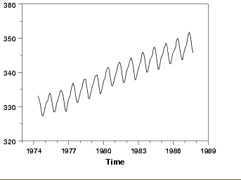

It is important to know about stationarity because of the fact that without a stationary series we cannot move forward with time series analysis.

We’ll need to calculate the mean of a time series in order to estimate the expected value. But, if the time series is not stationary then our calculation for expected value will give false results and interpretation.

Now, if a series is not stationary then we will need to convert the non-stationary series into a stationary series. In order to do this, we’ll have to differentiate the series.

White Noise:

• Apart from a stationary series, A white noise series is a series where the mean and variance of the data points is constant but there is no Autocorrelation between values of those data points.

AutoCorrelation:

• The correlation between values of data points at different time intervals is known as Autocorrelation. It is also sometimes termed as Lagged Correlation.

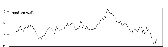
Now, when the mean and variance of time series data is not constant i.e. varying with time, then we can say that the data is just taking a random walk with time.

Random Walk:

• Random walk is a term used when data points in the series are not dependent on their past values. This makes the series Non-Stationary Series because the mean and variance will vary with time.

Visualizing Time Series Data: in R & Python

In order to visualize a time series data, we’ll make use of libraries Plotly for Python & timeSeries for R

Python:

Let’s begin with the python code for Time Series data visualization

We’ll use the following dataset for visualization. we’ll make use of the Date and AAPL.Close column for the visualization purpose.

The following python code is used for plotting. It shows the variation of close price over different time intervals.

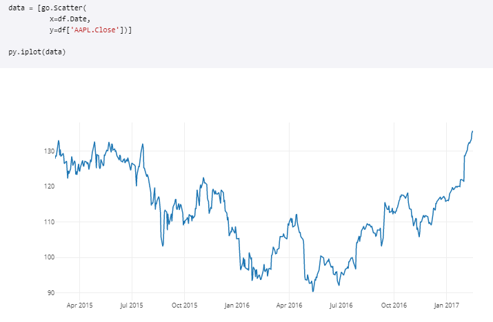
To find out more ways of plotting a Time Series, Have a look at ploty’s official documentation

R:

We’ll use inbuilt Air Passengers dataset from R and visualize time series data.

The dataset shows the number of passengers travelling on a flight for all the months in a year.

Below plot shows how they vary with time.

By now, you must be familiar with how a Time Series Data looks like. So next, we’ll study about different components in a time series data.

Components of Time Series:

Now, as we know that a time series data varies with time, there are many factors which results in this variation.

The effects of these factors are studied by following four major components:

• Trends
• Seasonal Variation
• Cyclic Variation
• Irregular Variation

Trends:

• The variation of observations in a time series over a long period of time is known as Trends. Thus, a Trend won’t bother about any short-term variations in the data.

For Eg:

1. Increase in Population
2. Increase in Gold Rates
3. Decrease in Death Rates

• Any time series which is gradually increasing or decreasing over a long period of time is said to have Trend.

Seasonality:

• The variation of observations in a time series caused due to regular or periodic time variations is known as Seasonality.
• A repetitive pattern that can be predicted is termed as Seasonality. It also considers the short-term fluctuations in time.

For Eg:

1. Travel during holidays
2. Density of mosquitoes in winter
3. Ice cream sale in summer

Cyclic Variation:

• The variation of observations in a time series occurring generally in business and economics where the rises and falls in the data are not of fixed period is known as Cyclic Variation.
• The duration of these cycles is more than a year.

For Eg:

1. Sensex Price

Irregular Variation:

• The variation of observations in a time series which is unusual or unexpected is known as Irregular Variation.
• It is also termed as a Random Variation and is usually unpredictable.

For Eg:

1. Strikes
2. Natural Disasters

Time Series Modelling:

There are various techniques for time series modelling. Let us go through them one by one.

Auto-Regressive Model (AR):

AR model is a type of time series modelling where the value of a series at any point of time is only dependent on its past values. A point Y(t) can be said to have dependent on it values at Y(t-p) where p defines the number of past values (LAG).

Moving Average Model (MA):

MA model is a type of time series modelling where the value of a series at any point of time is only dependent on random error term which follows a white noise process. In laymen terms, A moving average is a time series constructed by taking averages of several sequential values of another time series. Here we’ll use the error terms from the regression instead of its past values.

Combining both AR & MA, ARMA and ARIMA are used for time series forecasting.

ARMA:

ARMA is the combination of both AR & MA where the value of a series at any point is dependent on its past values as well as the error terms.

These models such as AR, MA and ARMA are used when data is stationary.

Stationarity Check:

In order to check if a series is stationary or not we use Ljung-Box test or Augmented Dickey-Fuller Test.

Here, we observe that the p-value < 0.05. Hence, we can say that the series is stationary.

Now, If data is not stationary then we have to make the data as stationary by differentiating. For this kind of data, we use Autoregressive Integrated Moving Average(ARIMA).

Autoregressive Integrated Moving Average(ARIMA):

ARIMA is generally represented as ARIMA(p,d,q) where,

• p is past values
• d is differentiating order
• q is error term

To find optimal values of ARIMA model, we will use ACF and PACF.

Autocorrelation Function (ACF):

ACF is the coefficient of correlation between the value of a point at a current time and its value at lag p. i.e. correlation between Y(t) and Y(t-p)

We should calculate ACF in order to know up to what extent current values are related to the past values. Thus, we can know which past values will be most helpful in predicting future values.

Partial Autocorrelation Function (PACF):

PACF is same as ACF just that the intermediate lags between t and t-p is removed i.e. correlation between Y(t) and Y(t-p) with p-1 lags excluded.

We’ll plot ACF as well as PACF in R

Here, we can see that the ACF is not well within the confidence interval band. Hence the series is not stationary. We’ll differentiate the series once and observe the results.

Now, our series is stationary as most of the spikes are within the boundary. Thus, the value for I will be 1.

Also, the value of ACF at lag-1 is out of boundary, thus value of p should be 0.

Now,we can fit ARIMA on the time series data.

arima(AP,order = c(0,1,1))

We can try different combinations for q and check out for AIC, BIC values for each model. The model with the lowest AIC is the correct model.

To automatically choose best values for p,q and d, we can use auto.arima.

auto.arima(AP)

After fitting the best model, we check for randomness. tsdiag() produces a diagnostic plot of a fitted time.

tsdiag(auto.arima(AP))

Next, we’ll predict the values for next 8 time intervals, i.e. next 8 months.

predict(auto.arima(AP),n.ahead=8)

The output of predict will contain two lists. Predicted values ($pred) and standard errors of prediction ($se)

Conclusion:

With this blog you must have gained a comprehensive knowledge of Time Series Analysis and it’s implementation in R. Try to explore more with different time series data and interpret your results.

Here is a comparative study on correlation and regression that you can use to clear your understanding.