Top Excel Interview Questions and Answers to Crack Job Interviews

Excel Interview Questions and Answers

When you are interviewed for a job, there is a high possibility of Microsoft Excel interview questions and answers being asked. To help you prepare, we will cover a few basic Excel interview questions and answers,  and even some advanced Excel interview questions and answers.

Q1.) What is the difference between absolute and relative cell references?

Some basic Excel interview questions and answers are very likely to include something on cell referencing / locking.
For example, when you write in=A2+10 a cell and copy the formula down, in the next cell it will become=A3+10 This is a Relative cell reference – relative because of the reference changes when copied somewhere else. If we put dollar signs before each part of the reference,=$A$2+10 it becomes an absolute / locked reference. If this is copied down, it will stay the same and will not change to A3.
To illustrate the use of both types of references, let’s take a simple scenario where all the employees of a company are to be given a couple of bonuses. Some of the employees are to be given a 15% bonus for excellent performance. There is also a 10% bonus for an upcoming festival which will be given to all employees.

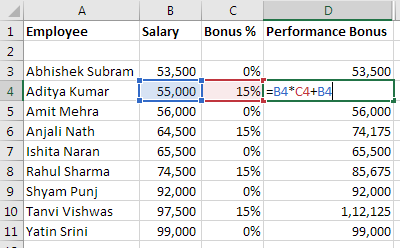
Here, all the cell references are relative. Which means, when this formula is copied down for each employee, the cell reference will change its position for each row. So, the references B4 and C4 will become B5 and C5 when copied down.

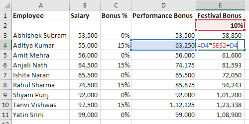
Here, since the 10% is fixed, the reference to it should also be fixed. If not fixed, it will keep changing. To prevent it from changing position, the reference is made absolute by putting the dollar signs before the alphabet and the number. In the screenshot above, the E2 is changed to $E$2. The reference to D4 is left relative so it changes in each row, when copied down.

Q2.) How and why to use advanced filters?

Advanced filters are used to filter using complex criteria. The key requirement is a proper dataset:

• A proper dataset is labelled with appropriate headers.
• It grows vertically (meaning, no new columns need to be added).
• It also has no empty rows or columns.

To use advanced filters, first list out the criteria required for filtering any column(s) like so:

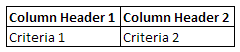
This is why the label headers are important. You can list down any number of columns with respective criteria like this. Next, click somewhere in the dataset and go to Data Tab and click on Advanced Filter in the Sort & Filter group (or press Alt - A - Q). We will filter the list in place and select the range of criteria – with the headers:

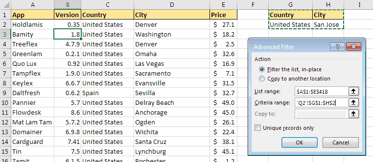
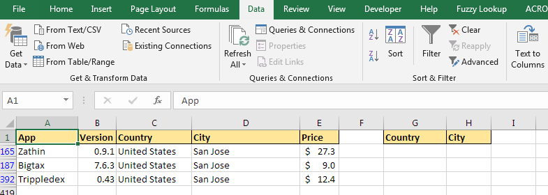
Pressing ok will filter the list to only show records that fulfil the criteria.

Advanced filters are useful because:

• They are easier to use with multiple criteria
• They allow for use of ‘and/or’ filtering. For example, with normal filters, there is no way to show only those records where the country is “United states” AND the city is “San Jose”. But with advanced filters, it’s a matter of putting both on the same row.
  If you put 2 criteria on different rows, the filter will show only those records where either the first OR the second criteria is met.
• They can also be used to show unique values – just turn on “Unique records only” in the options – no criteria is to be specified for this.

Q3.) Give 5 differences between Google sheets and Excel.

1. Google Sheets is free, Excel is not
2. Easy collection & collaboration in Google Sheets. Difficult collaboration in Excel
3. Clear revision history in Google Sheets. Excel requires manually saving each new version.
4. Excel is more capable of heavy calculations and data models. Google Sheets tends to slow down when many complex calculations are added.
5. Excel has tools like What-if Analysis. Google Sheets has functions like GoogleFinance, Sort, Filter, Query, Import Functions, etc. that are not available in Excel.

Q4.) What are the kinds of charts available in Excel? Which are the new ones available in Excel 2013/2016 version?

Ms Excel interview questions and answers might include general knowledge questions like this. Here are the chart types available:Before Excel 2016

Q5.) How to make dynamic drop down list?

The easiest way to make a dynamic drop-down list is by using the auto-expanding feature of Excel tables. Steps to do so:

1. First, make your list then press control + T to convert it into a table (without headers).
2. Then, select a cell/range where the dropdowns are to be made.
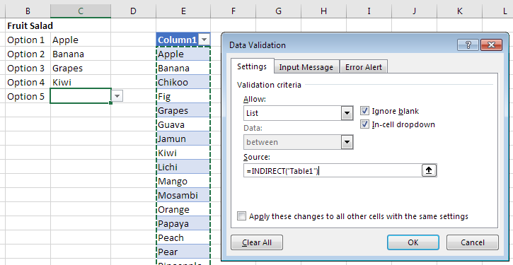
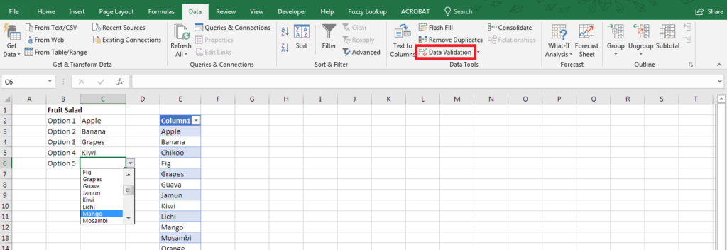
3. Next, go to the data tab and select data validation.
4. From there, under ‘Allow’ select ‘List’.
5. In the source put the Indirect function with the name of the table like so =INDIRECT("Table1"). The name of the table can be seen/edited in the design tab, after you click inside the table.

This function basically converts a reference that is plain text to one that is readable by Excel. Now, whenever the table is updated, all lists referring to it will also contain all new items automatically.

Q6.) What are the uses and limitations of vlookup?

Vertical – Lookup is basically used to extract values from a dataset, based on a given criterion. It can be used in many ways like:

• Searching & Extracting records/details from a dataset
• Comparing lists for common items
• Combining / Merging datasets based on a common column
• Grade or classify within ranges – like age groups, or tax brackets

It has some limitations like:

• Can only search in the first (leftmost) column
• Only looks right, so it cannot be used to search to the left.
• Only finds the first match. All others are ignored.
• Is fragile – Inserting/deleting a column in the table_array might break existing Vlookups

Q7.) What is a Pivot table & why is it used?

A pivot table is a feature in Excel that is used to summarise data into reports. Each column in the data becomes a “Field” in Pivot tables. These fields can then be arranged into rows & columns. All numerical “values” can be easily summarised and calculated. All this can be done in a few seconds as it is only a question of dragging and dropping fields into place. Using this you can quickly create reports that answer business questions – analysis of data becomes a breeze. To see a few of the reports that can be made using a single, proper dataset, let’s take an example of sales data:

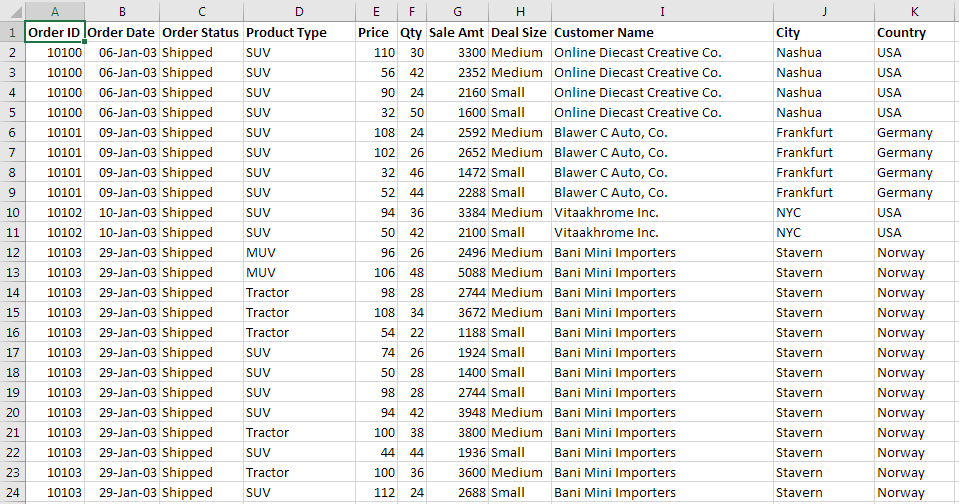
Here, each row contains a single order with every detail filled in. Using this the following reports can be easily made:

• Total sales for each Customer
• Number of Orders for each order status
• Quantity or sales for each product type
• Number of orders for each deal size
• List of Customers
• Number of Customers from every country
• Sales in each quarter
• Yearly Sales
• Seasonality of sales

These can be used to answer many business questions and analyse data better.

Q8.) Is it possible to make Pivot Tables using multiple sheets of data? How?

Some advanced Excel interview questions and answers might include this kind of question.

Yes, it is possible. There are 2 ways to do so, depending on the structure/layout of data. If the multiple sheets of data are in the same structure/layout, they can be consolidated into a single pivot table. If not, relationships have to be created between the datasets to create a relational database in Excel.

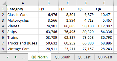
Method 1 – Consolidation

Use if  the data is in different sheets, having the same layout:

This is done by using the hidden (legacy) Pivot Table Wizard in Excel to combine all the data.

Steps:-

1. To open the pivot table wizard, use the keyboard shortcut Alt - D - P (in succession).

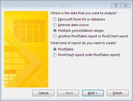
2. Select ‘Multiple Consolidation Ranges’
3. Next, select ‘I will create the page fields’
4. Next, Select each range and click ‘Add’ one by one. You will see the list is populated with whatever ranges you have added.
5. Click next and choose where you want to place the combined pivot table.

Method 2 – Relational Database in Excel

The other type is possible only in Excel 2013 or later. It uses a feature called Data Model. A data model basically lets you build relations between datasets. For this to happen, there must be a common column between 2 datasets. This common column is called, in data parlance, a ‘primary key’.

Let’s take a simple example using the data shown in the previous question. The same data is split into 3 sheets –
1. Invoices:

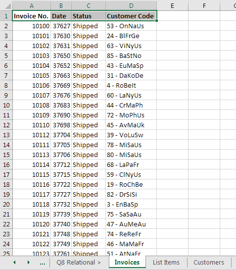
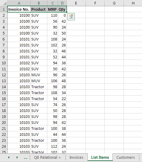
2. List Items:

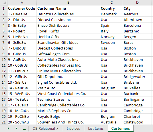
3. Customers (with some adjustments):

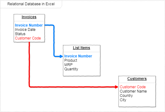
To use these together in a single pivot table, the common columns between them need to be linked to each other:

To do so, follow these steps:

1. Convert all 3 datasets into Excel tables (Ctrl + T)
2. Rename all tables appropriately (Click inside Table > Design > Table Name)
3. Insert a Pivot Table for the first one and select “Add this data to the Data Model”
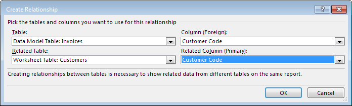
4. Go to the Analyze Tab (available when active cell is in a pivot table area) and choose “Relationships”. In the dialogue that pops up, click on “New”. This is where common columns are specified. This has to be done twice. One relationship will be from Invoices to List Items and the common column will be Invoice Number.

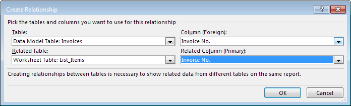
The second relationship is from Invoices to Customers; and the common column is Customer Code. Once done, close the Dialogue box.

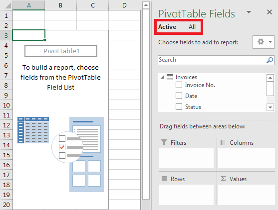
5. Next, in the pivot tables field list, go to the “All” section. You will see a list of the other two tables. Right – click each & choose “Show in Active Tab”.

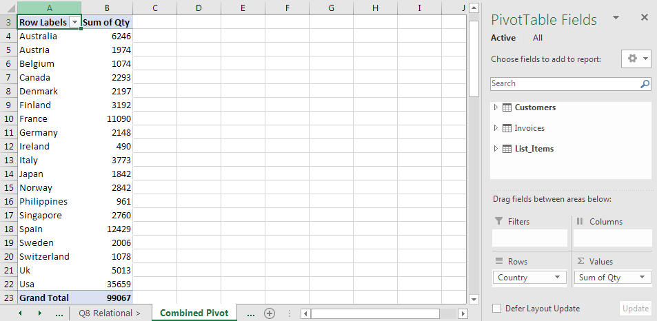
6. Done! Now if you go to the active tab, you can use pivot tables normally, while using fields from all the three datasets!

Q9.) What are macros used for?

Macros are pieces of code used to automate tasks & processes in Excel. These can be made by either recording or writing out VBA code (Visual Basic for Applications). As a recommendation, any fixed, repetitive tasks can and should be automated using macros.

For instance, if you need to keep importing data from a backend system into Excel. Every time you import, the data needs to be cleaned and formatted in the same way. This is a situation where you can write or record a macro once, and just click a button to run it every time new data is to be imported. VBA is also used to create define your own functions.

Q10.) Talk about some of the spreadsheets you’ve made that you’re most proud of.

MS Excel interview question and answers might easily include something like this. So, before looking for a job, make sure you build something challenging on your own. This will ensure you have hands-on, practical knowledge that is sure to land you a Job!

Ready for Interview?

The list of top Excel Interview Questions and Answers will help you face interview panel with great confidence.

If you wish to establish or accelerate your career in Data Analytics, then investing in a clear & comprehensive Data Analytics Techniques for Excel course would be one of the best investments you could make.