
Vlookup is a built-in function in Excel found under the Lookup & Reference tab. Vlookup performs a vertical search in the first column of a table and returns the value in the same row on the right.
Vlookup is best used when you have a vertical alignment of data sets in a structured table, and a column on the left which you can use to match a row.
Once you understand what Vlookup is, it is quite easy to use.
What Is Vlookup in Excel?
Vlookup is an Excel function, that, as the name suggests, is used to look up and retrieve data from a specific column in an Excel table.
Vlookup supports approximate and exact matching and uses wildcards for exact matching.
So, what is Vlookup used for? Vlookup is used to match a value in the first column and get the lookup value in the second column.
Using Vlookup, you can retrieve data from vertical columns in excel, which is what the “V” in Vlookup denotes. Here are a few more features of Vlookup.
Vlookup only works on the right
When using the Microsoft excel Vlookup function, the values for which you want to find a lookup should be in the left column, and the Vlookup data will appear in the right column.
Vlookup uses numbers not alphabet
When entering the Vlookup column, you need to specify the column number rather than its alphabetical value.
Vlookup has an exact and approximate match
There are two matching modes in Vlookup, exact and approximate. Users need to specify the kind of match they want when entering the lookup values.
Exact Match: This mode is used in most cases. Users look for an exact match when they have a unique key to search against.
Approximate Match: This mode is used when you are searching for the best match and not an exact match of a value.
Now that you have an idea of what is Vlookup, let’s look at the syntax and uses of Vlookup.

Syntax and Parameters for Vlookup
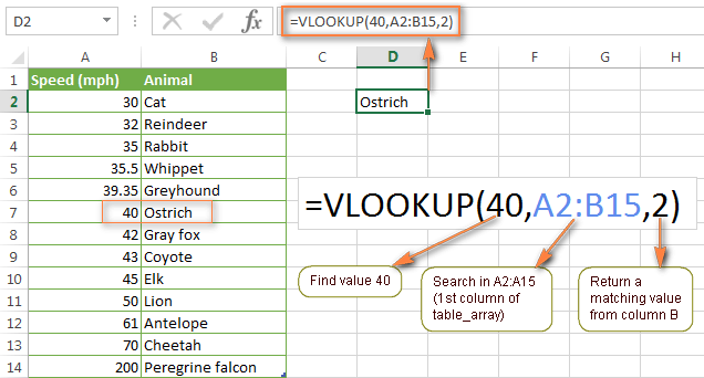
The correct syntax for using Vlookup in Excel is VLOOKUP(value, table, index_number, [approximate match]). But, just getting the syntax right is not enough to get the Vlookup value.
So, what is Vlookup influenced by? There are various other parameters and excel functions that need to be appropriately configured. First, let’s look at what each value in the Vlookup syntax stands for.
Argument Parameters
Value: This is the value you will be searching against the Vlookup.
Table: The set of data containing two or more columns to be used for looking up data.
Index_number: This is the column number in a table for which the matching value is to be derived.
Returns
You can get any data type from the Vlookup function, including string, number, or data.
To get the approximate value for your data, specify TRUE in the match parameter, and if no matching value is found, you will get the next closest value. Similarly, if you specify TRUE for the match parameter, the result will be N/A, if there is no matching value.
Let’s understand the syntax with an example.
First Parameter
This parameter is the value you need to search for in the lookup function. Say your first parameter is the id number 11. So, Vlookup will search for this value in the first column of the data.
Vlookup needs numeric values only, and since the id number is a numeric value, it can be added as-is. If it were a text, you would have to put it in double quotes, for example, “text”.
Second Parameter
This parameter is the source of the data where the vertical lookup will be performed. Say your second parameter is A1: B3, you would have two data columns to use in the lookup.
Here, the first column is the id value “11” and the second is the value to return.
Third Parameter
This is the position number in the table where you will get the return data. If you say “1”, it signifies the first column in the table, the value “2” signifies the second column, and so on.
Fourth Parameter
This is the last parameter in establishing your Vlookup function. Using this parameter, you can specify that you want an exact or approximate match, and the exact or approximate value matches can be configured by the user with TRUE or FALSE values.
How to Use Vlookup in Excel?
Vlookup is one of the most Useful Excel Function for Data Scientists. And, using the Vlookup function is also simple with the right syntax. Thus, knowing how to use vlookup in excel is an added advantage.
If you know what product you are looking for, for instance, you want to find out the price of something, and you can enter the product name in Excel and Vlookup will find the price for you.
The following Vlookup YouTube video will explain everything about it, vlookup range, approximate matches and other key concepts-
The following steps will help you understand what is Vlookup and how to use it.
(i) First, click the cell where you want to calculate the Vlookup formula.
(ii) Then click the formula at the top of the screen in the menu bar.
(iii) On the ribbon that appears, click the dropdown arrow for Lookup & Reference.
(iv) In the menu that appears, click Vlookup.
(v) Now mention the cell where you want to enter the value of the data that you are looking for. Say, your cell is H2, so input “H2” in the lookup_value box.
(vi) Specify what data you want Vlookup to use in the table array box. You can select the entire table or a set of cells.
(vii) In the col_index_no box, mention the column number Vlookup will use to find your data. Vlookup asks you to use the numeric value of a column instead of an alphabetical value, so if your column is “C” use the value “3”.
(viii) Next, you need to clarify if you need an exact match by entering FALSE or TRUE for an exact match or approximate match, respectively.
(ix) Now, click OK at the bottom of the window.
(x) Once the Vlookup is entered, Excel will return the value you are searching for in cell H3 when you type the product in H2.
Analysis
This is the basic search functionality Vlookup offers. But, what is Vlookup known for is its ability to allow users to combine two worksheets into one to search for values.
Say you have names in one worksheet and contact details in another worksheet, you can add the contact details next to the names with Vlookup.
Vlookup is a useful Excel function using which users can leverage their spreadsheets’ data for outside sources. No matter what field you are working in, it can help you find data.
But remember, when working with Excel formulas and functions, be careful about deleting columns. Say you emit a column when calculating Vlookup, then copy the Excel table into another worksheet, deleting a column will return an error.
10 Things You Should Know About Vlookup in Excel
Vlookup is used almost everywhere because of its ability to dynamically lookup data. It is a great feature when you want to pull up information from an excel worksheet quickly and comes when it comes to Data Analytics using Excel.
Here are the top Vlookup features you should know about.
1. Vlookup allows merging data
Vlookup is commonly used to join data from two or more tables. Like the example we saw earlier, say you want to match names to contact details, you can use a common id to pull up the data in the other table.
To enable this, you need to configure Vlookup to use the id value in one table and the corresponding data in the other table.
2. You can categorize data with Vlookup
Vlookup function allows you to apply arbitrary categories to your Excel table. Assign the categories using the table that acts as a “key” to assign the categories.
For example, you want to assign a grade based on a score, and you can configure Vlookup to assign an approximate match. Also, make sure that your table is sorted in ascending order to get the approximate right match.
3. The default match is approximate
Range lookup controls the exact and approximate match in Excel. The default in this range argument is TRUE, which means you will get an approximate match every time you apply Vlookup.
To get an exact match, set the range argument to FALSE, or zero. This will get you the exact match in Vlookup, and if no exact match is found, it will return the value as N/A.
4. Vlookup is made portable with absolute references
When you want to get data from more than one column in a table, use the absolute references for the table array. This also works when you want to copy and paste a Vlookup.
To do this, copy the formula and change the column index number so that you can use the same lookup value from a different column.
5. Name ranges to make reading Vlookup easier
Absolute ranges can look like disarray and using named ranges will make it easier to read your data by making it appear cleaner.
Replace absolute references with named ranges, which are automatically absolute. Say you add id before a name column and name the data in the table as “data,” your formula will be “=VLOOKUP(id,data,4,0), where 4 and 0 are the column numbers.
This also makes your data more portable.
6. Inserting a new column can break existing Vlookup
When you already have existing Vlookup formulas, adding a new column will break the formula. Hard-coded column values don’t automatically change when columns are inserted or deleted.
To avoid this, you can calculate a row or column to calculate a column index. Use the COLUMN function to generate a column index.
7. Enable partial matching with wildcards
If you are using Vlookup for an exact match, you have the option to use wildcards for partial matching. These wildcards will allow you to do an exact match based on a partial match.
You have two wildcard characters in Excel: an asterisk (*) to match one or more characters; and a question mark (?) for matching one character.
8. Trap N/A errors to display a message instead
When using an exact match, Vlookup will display an exact match when no exact match is found. While this lets you know that there is no match for a value, looking at an N/A error is not fun to look at.
To catch this error and display a message instead of “N/A” wrap the original formula in IFERROR and set the result you want, like a “not found” message.
9. Using numbers may cause text errors
If your table in Vlookup has numbers in the text area, you will get a N/A error when you run Vlookup.
So, to avoid this, ensure that the lookup value and the first column have the same data type, where both can be either numbers or text.
10. Vlookup can replace nested IF
When asked what is Vlookup most used for, the answer would be to replace nested IF statements. A series of nested IFs may look fine, but they require parenthesis wrangling.
Just make sure that the right key table is set up for Vlookup, that is it contains brackets to handle your values. When anything in your table changes, you can simply update the table and the Vlookup formulas will update too.
Xlookup vs Vlookup
You’ve probably seen the terms “vlookup” and “xlookup” before, but what do they mean? And more importantly, which one should you use? Let’s take a look at the differences between vlookup and xlookup to help you make the best decision for your needs.
Vlookup stands for vertical lookup, and it is the traditional way of looking up data in Excel. With vlookup, you specify a value to look for in the first column of a table, and then Excel returns the value from another column in that table.
Xlookup is a newer function that was introduced in Excel 2019. It offers a few advantages over vlookup, including the ability to look up values in a table that is not sorted and the ability to return multiple values.
Here’s a quick rundown of the main differences between vlookup and xlookup:
- Vlookup can only look up values in the first column of a table. Xlookup can look up values in any column.
- Vlookup can only return values from the same row as the lookup value. Xlookup can return values from multiple rows.
- Vlookup requires the table to be sorted in ascending order. Xlookup does not require the table to be sorted.
- Vlookup can only return a single value. Xlookup can return multiple values.
So, which one should you use? If you’re using Excel 2019 or later, xlookup is a clear choice. However, if you’re using an earlier version of Excel, vlookup is still a perfectly good option.
Vlookup example between Two Sheets
When you have your data in two different worksheets, you can use vlookup to search for a specific value in one sheet and return a corresponding value from the other sheet. This is especially useful when you have large amounts of data in different worksheets and need to consolidate them into one master sheet.
To do this, you’ll need to use the vlookup function with the following syntax:
=VLOOKUP(value, sheet1!range, column, FALSE)
Value is the value you want to search for in sheet1.
The range is the range of cells in sheet1 that contain the data you want to search. This can be a specific range (like A2:F10), or the entire column that contains the data (like A:F).
The column is the column number in sheet1 that contains the value you want to return. For example, if the value you want to return is in column 2, this would be 2.
FALSE indicates that you want an exact match. If you use TRUE, vlookup will return the closest match.
For example, let’s say you have a list of names and phone numbers on one sheet and a list of names and email addresses in another sheet. You can use vlookup to search for a specific name in the first sheet and return the corresponding email address from the second sheet.
In the first sheet, the list of names and phone numbers looks like this:
A B
Name Phone Number
John 555-1212
Jane 555-1313
Joe 555-1414
In the second sheet, the list of names and email addresses looks like this:
A B
Name Email Address
John john@example.com
Jane jane@example.com
Joe joe@example.com
To use vlookup to return the email address for Jane, you would use the following formula:
=VLOOKUP(“Jane”, Sheet1!A:B, 2, FALSE)
This would return “jane@example.com” from the second sheet.
Vlookup formula pdf:
As it is clear that Vlookup is a function in Excel that allows you to search for a value in one table and return a corresponding value from another table.
The “v” stands for “vertical”. This is because the function is designed to work with data that is arranged in columns. You can use the vlookup function to search for a particular value in a column of data and return a corresponding value from another column.
For example, you could use it to search for a customer’s name in a list of customers and return the customer’s ID number. The vlookup function is one of the most popular functions in Excel. It is a versatile function that can be used in a wide variety of situations. The vlookup function is available in all versions of Excel.
Conclusion
Excel is a primary application used by Data Analysts, and hence, they need to know the proper way to use the tool.
Having a thorough understanding of what is Vlookup can help you retrieve and analyze data better.
The Certified Data Analytics Course will help beginners get to gain more analytics skills and build a career as a Data Analyst.
What is Vlookup in Excel FAQs:
Question: What is vlookup in excel with an example?
Answer: When it comes to understanding what is Vlookup in excel, you need to understand it as a function in excel that allows you to search for a value in one table and return the corresponding value from another table. For example, you can use vlookup to search for a customer’s name in a list of customers and return the customer’s address.
Question: What is the syntax of vlookup?
Answer: The syntax of vlookup is as follows:=VLOOKUP(value, table, col_index, range_lookup)
Question: What are the arguments of vlookup?
Answer: The arguments of vlookup are as follows:
- Value: the value that you want to look up. This can be a number, text, or a reference to a cell containing the value that you want to look up.
- Table: the table of data that you want to search. This can be a reference to a range of cells or an array constant.
- Col_index: the column number in the table that contains the value that you want to return. For example, if the value you want to return is in the second column of the table, you would use a col_index of 2.
- Range_lookup: a value that specifies whether you want vlookup to find an exact match or an approximate match. If you specify TRUE or omit this argument, vlookup finds the closest match in the first column of the table. If there is no exact match, the next largest value that is less than value is returned. If you specify FALSE, vlookup only returns an exact match. If an exact match is not found, #N/A is returned.
Question: What is the difference between vlookup and hlookup?
Answer: Vlookup is a function that searches for a value in the leftmost column of a table and returns the corresponding value in the same row from another column in the table. Hlookup is a function that searches for a value in the top row of a table and returns the corresponding value in the same column from another row in the table.
Question: How to use vlookup in excel 2022?
Answer: You can use vlookup in excel 2022 by following these steps:
- Enter the value that you want to look up in the first column of the table.
- Enter the table of data that you want to search in the second column of the table.
- Enter the column number in the table that contains the value that you want to return in the third column of the table.
- Enter a value of TRUE or FALSE in the fourth column of the table to specify whether you want vlookup to find an exact match or an approximate match.
- Press Enter and the vlookup function will return the value that you specified.