
Travis Oliphant invented NumPy by combining the features of Numarray and Numeric, together with his own modifications. Numpy is open-source software with a number of contributors. Let’s learn through NumPy Tutorial.
Before we begin with the Numpy tutorial, we need to understand that when people initially work with NLP (Natural Language Processing), they use default Python lists.
With time, however, they shift to Numpy. This is because bigger experiments that involve lots of data are not always amenable with default python lists. Python lists tend to use up too much RAM which is where Numpy comes in.
The Numpy Tutorial: What is a Numpy Matrix?
Numpy means Numerical Python. The Numpy matrix is a package in Python which is the core scientific computing library. It contains a powerful n-dimensional array object and also enables integrations of C and C++.
The Numpy matrix has a number of uses; from linear algebra to random number capability to its use as a container for generic data. You can check out this video for a Numpy tutorial that covers the basics about Numpy.
NumPy Tutorial: Installing NumPy
All you need to do is type “pip install numPy” in the command prompt. This starts the installation. As soon as Numpy is installed go to the IDE(Integrated Development Environment) and then import Numpy by typing “import NumPy as np”.
NumPy Tutorial: NumPy Array
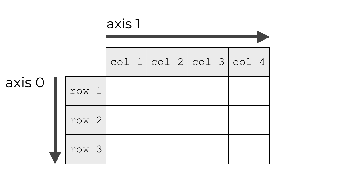
A Numpy Array or Numpy matrix is a two-dimensional array that contains both rows and columns. Here’s an example of a NumPy array that has 4 columns and 3 rows.
Numpy Tutorial: Implementing Numpy in PyCharm
This is how you can implement the Numpy matrix in PyCharm (one of the most commonly used IDEs):
Single-Dimensional Numpy Matrix:
|
1 2 3 |
import numpy as np a=np.array([1,2,3]) print(a) |
Output – [1 2 3]
Multi-Dimensional Numpy Matrix:
|
1 2 |
a=np.array([(1,2,3),(4,5,6)]) print(a) |
O/P – [[ 1 2 3]
[4 5 6]]
Numpy Tutorial: Python Numpy Matrix vs Python list
Most people prefer using Numpy to the default Python Data lists especially when it comes to complex operations that involve large amounts of data. Here are some reasons why:
(i) NumPy is much faster than default lists when it comes to executing data models.
(ii) It is better optimized and requires less RAM than Python lists. That’s why most data scientists prefer using it when the volumes are large.
(iii) NumPy has a learning curve but it is also more convenient to use than lists in the long run.
Best Numpy Tutorial: Important Operations
Just like the arrays in C, you have to create NumPy arrays in advance and then just fill them. Of course, this means you can’t merge or append arrays in Numpy because you’ll get one array in the size of the contents of the arrays that are getting merged. Then the contents of the arrays will get copied onto this one array.
Here’s one of the best Numpy tutorials to highlight some critical operations that can be done using NumPy.
Numpy Python Tutorial: How to Create ndarray
Learn here how you can create a NumPy array using different methods.
(i) Numpy Tutorial: How to create a NumPy matrix in the same shape but as a different array. This uses the function NumPy.empty_like():
# Creating ndarray from list
c = np.array([[1., 2.,],[1., 2.]])
# Creating new array in the shape of c, filled with 0
d = np.empty_like(c)
(ii) Then you cast the NumPy array from the Python list using the function NumPy.asarray() :
import NumPy as np
list = [1, 2, 3]
c = np.asarray(list)
(iii) You can also create a customized ndarray in the required size. You can fill it with random values, ones, or zeroes.
# Array items as ndarray
c = np.array([1, 2, 3])
# A 2×2 2d array shape for the arrays in the format (rows, columns)
shape = (2, 2)
# Random values
c = np.empty(shape)
d = np.ones(shape)
e = np.zeros(shape)
Numpy Python Tutorial: Slicing a NumPy Array
Some times, you may need to use only certain rows and columns instead of the entire array. To use only particular rows and columns, use the slicing feature. Here’s how:
a = np.asarray([[1,1,2,3,4], # 1st row
[2,6,7,8,9], # 2nd row
[3,6,7,8,9], # 3rd row
[4,6,7,8,9], # 4th row
[5,6,7,8,9] # 5th row
])
b = np.asarray([[1,1],
[1,1]])
# Select row in the format a[start:end], if start or end omitted it means all range.
y = a[:1] # 1st row
y = a[0:1] # 1st row
y = a[2:5] # select rows from 3rd to 5th row
# Select column in the format a[start:end, column_number]
x = a[:, –1] # -1 means first from the end
x = a[:,1:3] # select cols from 2nd col until 3rd
Numpy Python Tutorial: How to Merge Arrays
Instead of merging arrays, a better approach is to create an array of the size you need and fill it. This is because merging arrays only results in the creation of a big array and the copying of the contents into this new array.
If you do need to merge arrays, however, use these functions:
(i) Concatenate
1d arrays:
a = np.array([1, 2, 3])
b = np.array([5, 6])
print np.concatenate([a, b, b])
# >> [1 2 3 5 6 5 6]
2d arrays:
a2 = np.array([[1, 2], [3, 4]])
# axis=0 – concatenate along rows
print np.concatenate((a2, b), axis=0)
# >> [[1 2]
# [3 4]
# [5 6]]
# axis=1 – concatenate along columns, but first b needs to be transposed:
b.T
#>> [[5]
# [6]]
np.concatenate((a2, b.T), axis=1)
#>> [[1 2 5]
# [3 4 6]]
(ii) Append
Appending enables you to add values at the end of an existing NumPy array. Here’s how you do it:
1d arrays:
# 1d arrays
print np.append(a, a2)
# >> [1 2 3 1 2 3 4]
print np.append(a, a)
# >> [1 2 3 1 2 3]
2d arrays.
pend(a2, b, axis=0)
# >> [[1 2]
# [3 4]
# [5 6]]
print np.append(a2, b.T, axis=1)
# >> [[1 2 5]
# [3 4 6]]
(iii) Hstack (stack horizontally) and vstack (stack vertically)
1d arrays:
print np.hstack([a, b])
# >> [1 2 3 5 6]
print np.vstack([a, a])
# >> [[1 2 3]
# [1 2 3]]
2d arrays:
print np.hstack([a2,a2]) # arrays must match shape
# >> [[1 2 1 2]
# [3 4 3 4]]
print np.vstack([a2, b])
# >> [[1 2]
# [3 4]
# [5 6]]
(iv) linspace
Linspace returns evenly spaced numbers, spaced over a specified interval. For instance:
|
1 2 3 |
import numpy as np a=np.linspace(1,3,10) print(a) |
Output – [ 1. 1.22222222 1.44444444 1.66666667 1.88888889 2.11111111 2.33333333 2.55555556 2.77777778 3
Numpy Tutorial: Max/Min
This function helps us find the minimum and maximum values of a NumPy array.
|
1 |
import numpy as np |
|
2 |
a= np.array([1,2,3]) |
|
3 |
print(a.min()) |
|
4 |
print(a.max()) |
|
5 |
print(a.sum()) |
Output – 1 3 6
Numpy Tutorial: Square Root & Standard Deviation
The square root function returns the square root of every single element in the output. The standard deviation can also be returned. Let’s see how:
|
1 2 3 4 |
import numpy as np a=np.array([(1,2,3),(3,4,5,)]) print(np.sqrt(a)) print(np.std(a)) |
Output – [[ 1. 1.41421356 1.73205081]
[ 1.73205081 2. 2.23606798]]
1.29099444874
Numpy Tutorial: Python Numpy Special Functions
Mathematical functions like sine, tan, cos, log, etc can also be used you can use in NumPy. We can plot the sine, cos, tan function by importing Matplotlib. Here’s what it looks like for the sine function:
|
1 2 3 4 5 6 |
import numpy as np import matplotlib.pyplot as plt x= np.arange(0,3*np.pi,0.1) y=np.sin(x) plt.plot(x,y) plt.show() |
Output –
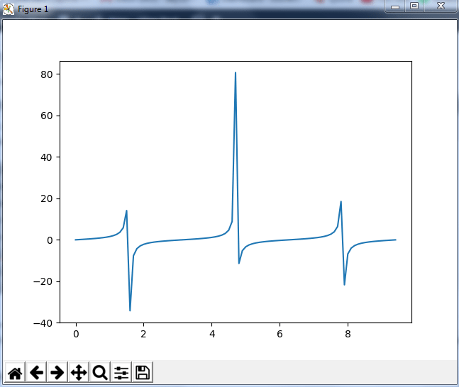
This is how we plot the tan function:
|
1 2 3 4 5 6 |
import numpy as np import matplotlib.pyplot as plt x= np.arange(0,3*np.pi,0.1) y=np.tan(x) plt.plot(x,y) plt.show() |
Output –
Conclusion
NumPy is far superior to default python lists and is a great tool for budding data scientists who want to perform more complex operations with large amounts of data.
There are many more operations that have not been discussed in this Numpy tutorial that can be executed with these Python Tools. Once you master the NumPy basics, you can move to more complex operations.
Are you also inspired by the opportunities provided by Python? You may also enroll for a Data Science Course for more lucrative career options in Data Science using Python.


Thanks for writing this in depth post. You covered every angle. One word to say, I love it!