
What Is Predictive Modeling?
Before we answer ‘what is predictive modeling’, let’s understand the basic uses of data. There are three most common uses of data: Analytics, monitoring, and prediction. Data Analytics is the use of past data to infer which event occurred, when it did, and why it did. Real-time Data Monitoring provides information and insights for live event tracking and detection, so proactive action can be taken. Predictive Data Modelling (also referred to as predictive analytics or predictive analysis) analyses past data to predict an outcome (a future outcome or an unknown past outcome). In this article, we will explore everything related to Predictive Modeling and clarify what predictive modelling is.
What Is Predictive Modeling?
Predictive modelling uses data and statistics to predict an outcome. This outcome can be in the future (which is most often the case), for example, the outcome of a sports game based on the past statistics of the teams involved, or it can be the unknown outcome of an event that has already occurred, for example in identifying a crime suspect based on existing data.
Predictive analytics has captured the support of a wide range of organizations, with a global market projected to reach approximately $10.95 billion by 2022, growing at a compound annual growth rate (CAGR) of around 21 per cent between 2016 and 2022, according to a 2017 report issued by Zion Market Research.
Here’s a video that explains the Difference between forecasting, Predictive modeling, machine learning.
How Does Predictive Modeling Work
A predictive modelling program is achieved via different algorithms (classification algorithms, clustering algorithms, regression algorithms, etc.) which use statistical models to accomplish the task. Before understanding the algorithms, let’s take a look at what statistical models are.
A statistical model uses a set of predefined assumptions to generate sample data from a provided larger data source. The sample data is the prediction that we look to extract. In short, a statistical model allows us to predict the probability of an event. There are two main types of predictive models (and hence two main classes of predictive models themselves) –
Parametric Statistical Models
Non-parametric Statistical Models
Parametric Statistical Models are those models that have a finite number of input parameters, and these are well defined. A simple example of this class is the Normal Distributions Curve (also known as the Bell Curve) as seen in the image below.
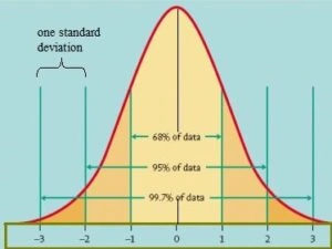
The normal distribution curve is derived from a finite set of initial parameter. To use this model as a prediction model, you just need to know the defined parameters and prediction can be made by plotting these parameters on the defined graph.
Non-parametric Statistical Models do not solely depend on the input parameters, mainly because the parameters do not have a normal distribution, and are hence not used for assumptions. For example, if you collect data of the time taken for different patients taking a particular drug to cure a cold, the data will not be normally distributed (because the cure time will be different for each patient, and also for the same patient when re-tested).
The type of statistical model forms the basis for the prediction model, and that depends on the type of data. Different predictive modelling algorithms have been developed, and the right algorithm depends on the data and the desired outcome. Let’s take a look at some predictive model types.
Predictive Modeling Techniques
Classification Predictive Modeling
This is the first of five predictive modelling techniques we will explore in this article. The Classification Model analyzes existing historical data to categorize, or ‘classify’ data into different categories. This model is best suited for ‘yes’ or ‘no’ scenarios, such as to check if a potential lead is going to convert or no, or if a loan is going to be approved or no, etc. The following are some important characteristics of a classification model:
A classification model is built from data that can be classified into two (or more) categories.
The data variables can be real values or discrete input variables.
A classification problem with two classes is called a two-class or binary classification problem, and one with more than two classes is called a multi-class classification problem.
A classification problem where the input variable is assigned more than one class is called a multi-label classification problem.
Most often, a classification predictive model predicts the class (‘yes’ an email belongs in spam or ‘no’ it does not) and not a continuous variable (like an integer), but it can be programmed to predict a continuous value as the probability, which can be correlated to an output class. For example, the threat level of an email can be measured between 0.1 to 0.9 (with step measures of 0.1) with 0.1 implying the email is less likely to be spam and 0.9 implying it is most likely spam. The prediction model, in this case, results in a continuous variable (a number between 0.1 and 0.9) which is translated into spam or not spam based on the result’s proximity to the lower and upper threshold. The algorithm can be built in many different programs and is a common example of predictive modeling in R.
The following article will help you understand classification better by taking the case of text classification: A Comprehensive Guide to Learning Text Classification.
Regression Predictive Modeling
A regression predictive model analyses input data to predict the required outcome, which is a continuous variable (or a real-value quantity and not just ‘yes’ or ‘no’) like an integer or a floating-point value. For example, the predictive model can analyze past real estate prices for a given location, and the movement in prices to predict the possible price of a house in that location, with the result being an actual monetary number (between Rs 75,00,000 and 90,00,000, for example). The following are some important characteristics of a regression model:
The input data variables can be real values or discrete input variables.
The output of a regression model is a quantity.
A regression model with multiple input variables is called a multivariate regression model.
A regression model where the input data is ordered by time is called a time series forecasting model.
The accuracy level of a regression predictive model’s prediction is measured by using the root mean squared error method. For example, if the program makes two predictions: Rs 1,000 when the expected value is Rs 1,200, and Rs 5,000 when the expected value is Rs 4,700, the error will be calculated as:
RMSE = sqrt(average(error^2))
RMSE = sqrt(((1200.0 – 1000.0)^2 + (4700.0 – 5000.0)^2) / 2)
RMSE = sqrt((40000.0+ 90000.0) / 2)
RMSE = sqrt(65000.0)
RMSE = 254.95
Like the classification model, the regression model is a common example for predictive modeling in R. here’s a knowledge article that will help you further understand regression models: A Beginner’s Guide to Understanding What is Regression.
Random Forest Predictive Modeling
Random Forest Predictive Modeling is one of the most commonly used predictive modeling techniques. It is capable of executing both classification and regression algorithms. The model gets its name because the algorithm is a combination of decision trees. Every individual decision tree is dependent on the values of a random vector that is independently sampled, and each tree is extended as much as possible. The following is an example of a decision tree (not the random forest predictive modeling):
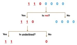
In the above example, the input data is split by applying filters at each node of the decision tree until we are happy with the final classification. We first split the data by asking ‘is the data red, and then by asking ‘is it underlined’. This gives a clear classification of 0s, 1s, reds and blues.
A Random Forest Predictive Model comprises many such decision trees. Each decision tree predicts an output class, and the majority is voted as the final result. This image will help you understand this concept:
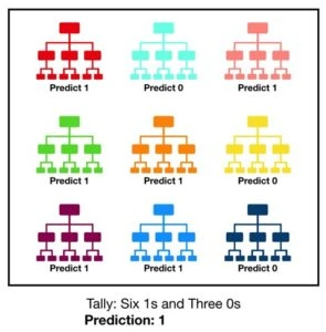
In this example, each decision tree within the forest predicts if the resulting class is a ‘1’ or a ‘0’, and the final output is the majority, which is ‘1’. A Random Forest Predictive Model reduces the chances of errors (as opposed to just using one decision tree as a predictive model) because the error made by one tree is diluted by other trees in the forest. Following are the benefits of the random forest model:
More accurate and efficient, especially when large databases are involved.
Having multiple decision trees reduces error possibilities and error variance.
The model can handle huge numbers of input variables without undergoing variable deletion.
Is capable of estimating which variables are important in classification.
Can be used to estimate missing data.
Following are the important features of a Random Forest Predictive Model:
It is made up of a large number of uncorrelated decision trees.
Each decision tree acquires data from the source by a method called ‘bagging’. This means each decision tree picks data from the original subset at random, further ensuring the different decision trees in the forest are uncorrelated.
The result is calculated at the end of the process, as an average or majority of the total results.
The higher the number of decision trees in the random forest predictive model, and the higher the uncorrelation between these trees, the higher the accuracy of the result. This model can be built via different programs, like predictive modeling in R.
Gradient Boosted Predictive Modeling
The Gradient Boosted Predictive Model is very similar to the Random Forest Predictive Model, in that it too uses decisions to make a prediction. The difference is in the method of using these decision trees, and the way the result is calculated.
The Random Forest Predictive Model used ‘bagging’ as a method to create the forest. Each decision tree independently and randomly selected initial data from the original subset to form the decision tree. The forest was made up of many such independent decision trees.
In the Gradient Boosted Predictive Model, each decision tree is built one at a time, with the results (the accuracy of the prediction) of one tree affecting the building of the next decision tree. This method of tree formation is called ‘boosting’ because each tree ‘boosts’ the next tree to provide better results. This is the first difference between the Random Forest Predictive Model and the Gradient Boosted Predictive Model, which is the formation of decision trees.

The next difference is the calculation of results. In the Random Forest Predictive Model, the results were calculated in the end by considering the results of all individual decision trees and taking an average or majority. In the Gradient Boosted Predictive Model, the results are calculated as the trees are built. The results of each tree weigh in on the building of the next tree, and the accuracy continuously improves.
Similar to the Random Forest Predictive Model, the Gradient Boosted Predictive Model has more accuracy than single decision trees, can accommodate huge amounts of data, and is one of the most commonly used predictive modeling techniques. This model can be built via different programs, like predictive modeling in R.
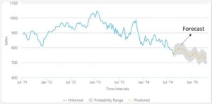
Time Series Predictive Modeling
The Time Series Predictive Model is built by capturing and plotting input data (historical data) based on time to predict the outcome for the foreseeable future. In simpler words, the Time Series Predictive Model can use the past years (arbitrary time value) data to predict the outcome for the next three months (arbitrary time value). The following examples should help you understand the use of this model: A company can use the sales data (like the number of calls received, the positive outcomes, negative outcomes, callbacks, etc.) for the past year to predict the number of sales they are likely to make in the coming month.
The model takes into account multiple factors that are fed into the algorithm and does not just predict based on averages. For example, a store owner can count the number of store visits they received the previous year and divide it by 12 to find the average store visitors and predict that as the visits they will receive the coming month. However, store visits are not a static number; they also depend on external factors like the season, holidays in the month, need for the product, etc. The Time Series Predictive Model is built to consider all desired factors and is much more accurate than calculating averages.
Benefits & Uses of Predictive Modeling
Predictive modeling is being actively used in multiple industries to gauge and predict future outcomes like customer acquisition, product demand, price fluctuation, etc. The following are some of the most popular uses and benefits of predictive modeling:
Customer relationship management
To predict the possible actions of a customer, usually in sales, marketing and retention.
Auto insurance
Policyholder data is analyzed to predict risk ratings for each member before assigning a policy.
Health care
Predictive analysis is used to forecast the chances of an illness recurring in a patient.
Trading
Programs with predictive modeling are being used to predict the movement of stocks to provide better chances of beneficial investing.
In every field that it is being used in, predictive modeling provides a forecast so proactive action can be taken. This is extremely beneficial in mitigating risks and putting precautionary measures in place.
As technology is progressing, predictive modeling programs are becoming more accurate and capable. The amount of data generated today is massive, and the growth in technology is providing higher computational power which means the machines today are capable of servicing and manipulating these large volumes of data for predictive analysis. Going forward, we will see technologies like AI, machine vision, and NLP greatly involved in predictive analysis.
Interested in Data Science? Here’s How to Build a Career in Data Science with Some Simple Steps.