One of the key challenges with any software program is optimization. The more we can optimize a program, the more efficient and accurate the output. One of the most popular optimization techniques in recent time is The Gradient Descent Algorithm.
Steve McConnell in his book Code Complete wrote: “The big optimizations come from refining the high-level design, not the individual routines.”
What is Optimization?
Optimization has applications across different fields from economics and mechanics to physics. However, it is in cutting-edge technologies like machine learning where optimization is the key to success.
Optimization means maximizing or minimising a function f(x). In machine learning, it refers to minimizing the cost or loss function J(w).
Most machine learning algorithms depend on optimization techniques including neural networks, linear regression, k-nearest neighbours, and so on. The gradient descent method is one of the most commonly used optimization techniques when it comes to machine learning.
What Is The Gradient Descent Algorithm?
A classic example that explains the gradient descent method is a mountaineering example. Say you are at the peak of a mountain and need to reach a lake which is in the valley of the mountain. Doesn’t seem that hard? Now imagine you are blindfolded and can’t see what’s ahead of you.
Instinctively, you will check the ground beneath your feet and figure out where it is going downward. If you keep following the path that is descending, you’re very likely to reach the lake at the bottom.

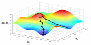
The above graph talks about this same gradient descent. Let us now understand how the gradient descent method applies to machine learning. Say you need the best parameters (θ1) and (θ2) for your machine learning algorithm.
You start by plotting the cost space. The cost space refers to how the algorithm will perform if you choose some value for the parameter. When you plot the cost space, you will find similar mountains and valleys as can be seen in the graph.
The cost J(θ) is mapped on the Y-axis against parameters θ1 and θ2 on the x-axis and the X-axis respectively. In this graph, the hills represent a high cost and are in red while the valleys, in blue, represent a low cost.
The different gradient algorithms are classified into two on the basis of the data being used to compute the gradient. In the case of the Full Batch Gradient Descent Algorithm, the entire data is used to compute the gradient. In Stochastic Gradient Descent Algorithm, you take a sample while computing the gradient.
Gradient descent algorithms can also be classified on the basis of differentiation techniques. The gradient is calculated by differentiation of the cost function. So the algorithms are classified on the basis of whether they use First Order Differentiation or Second Order Differentiation.
This video discusses the gradient descent machine learning algorithm and other optimization techniques.
What Are The Variants Of Gradient Descent Algorithm?
Here are some of the most commonly used variants of the Gradient descent algorithm. Each variant has its own specific use case.
(i) Vanilla Gradient Descent
Vanilla means plain and simple. And that’s why this technique is the simplest variant of the gradient descent algorithm. This technique involves taking small steps towards the minima by using the gradient of the cost function.
Here’s what the pseudocode looks like.
update = learning_rate * gradient_of_parameters
parameters = parameters – update
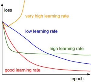
You use the gradient of the parameters and multiply it by a learning rate. A learning rate is a number which stays constant and indicates how quickly you want to reach the minima. Since the learning rate is a hyper-parameter it needs to be chosen carefully.
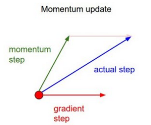
(ii) Gradient Descent With Momentum
The difference between this method and Vanilla Gradient descent is that this technique considers the previous step before taking the next one. This method has velocity, which considers the previous update, and constant momentum. This is the pseudocode:
update = learning_rate * gradient
velocity = previous_update * momentum
parameter = parameter + velocity – update
(iii) ADAGRAD
ADAGRAD uses an adaptive technique to update the learning rate, instead of keeping it constant. The learning rate changes based on how the gradient has been changing in the iterations that have taken place earlier. This is the pseudocode:
grad_component = previous_grad_component + (gradient * gradient)
rate_change = square_root(grad_component) + epsilon
adapted_learning_rate = learning_rate * rate_change
update = adapted_learning_rate * gradient
parameter = parameter – update
Here, epsilon is constant. It is used to keep the rate of change of the learning rate within limits.
(iv) ADAM
In a way, ADAM is a combination of momentum and ADAGRAD. Like ADAGRAD, it is an adaptive technique. It uses two constants, beta 1 and beta to keep both the rate of change of the learning rate and the changes in a gradient within limits.
This is the pseudocode.
adapted_gradient = previous_gradient + ((gradient – previous_gradient) * (1 – beta1))
gradient_component = (gradient_change – previous_learning_rate)
adapted_learning_rate = previous_learning_rate + (gradient_component * (1 – beta2))
update = adapted_learning_rate * adapted_gradient
parameter = parameter – update
Challenges In Executing Gradient Descent
The Gradient descent machine learning algorithm is one of the most successful optimization techniques with a proven track record. However, there are some cases where it becomes difficult to use. Here are some of the challenges with Gradient Descent.
(i) Improper execution of gradient descent can lead to issues like vanishing or exploding gradient. These usually occur if the gradient is either too large or too small. As a result, the algorithms don’t converge at the end.
(ii) You need to keep an eye on hardware and software considerations as well as floating-point requirements.
(iii) You need to make sure you have a good idea of the memory your gradient descent machine learning algorithm will require to execute. If you don’t have enough memory, the execution is likely to fail.
(iv) Gradient descent works only in cases where the convex-optimization problem is well-defined. If that is not the case, this optimization technique is unlikely to work.
(v) There can be points in the data where the gradient is zero but the point is not optimal. Such points are known as saddle points. This poses a major challenge to the efficacy of the method and no proper solution has been found so far.
(vi) During execution, you may come across many minimal points. The lowest of them all is the global minimum while others are local minima. It’s quite a challenge to make sure you find the global minimum and ignore the numerous local minima.
How To Choose The Right Gradient Descent Optimization Technique?
Every variant of the gradient descent algorithm has its own strengths and limitations. Choosing the right technique depends purely on the context. Here are some rules that you can use to make these decisions.
(i) The best results are obtained by the more traditional gradient descent optimization techniques. If you have the time and resources, use vanilla gradient descent or gradient descent with Momentum. While these techniques are slower, they are by-and-large more effective than adaptive techniques.
(ii) If you are at the MVP (Minimum Viable Product) stage and are looking to build rapid prototypes, adaptive techniques like ADAM and ADAGRAD are the better bet. You can get results faster with lesser effort. This is because adaptive techniques don’t require you to keep tuning the hyper-parameter.
(iii) Second-order techniques like I-BFGS are a great option if your data is small and doesn’t require multiple iterations. These techniques are both extremely fast and highly accurate. However, they don’t work on larger datasets that require more than one iteration.
What To Look Out For While Applying Gradient Descent?
There are some things you should keep in mind when applying gradient descent. If your machine learning algorithm is not working for some reason, these will serve as valuable checks.
(i) Check The Error Rates
Both the training and testing error should be checked after a certain number of iterations are complete. If both the error rates are not decreasing, there may be an issue.
(ii) Check The Gradient Flow In The Hidden Layers
If the gradient is too big or too small you might face a vanishing or exploding gradient problem. Check the flow of the gradient in the hidden layers to make sure this isn’t the case.
(iii) Keep A Check On The Learning Rate When You Use Adaptive Techniques
You need to keep an eye on the learning rate when you’re using adaptive techniques like ADAM and ADAGRAD. This is because these methods constantly update the learning rate and it’s important to keep it in check.
Conclusion
Gradient descent algorithms are the most tried and tested optimization technique when it comes to machine learning. A proper understanding of data science and machine learning algorithms is not complete without knowing how to implement gradient descent algorithms.
Of course, there are some things one needs to take care of while executing gradient descent algorithms. And there are particular situations in which this gradient descent optimization is not feasible. However, by and large, this technique is one of the most effective optimization techniques, especially for machine learning.
If you are also inspired by the opportunity provided by Data Science, enroll in our Data Science Master Course for more lucrative career options in the Data Science Landscape.