
There are many new algorithms and functionalities that come up in the evolving world of data science. Sometimes, algorithms that are not new are also used in interesting and unique ways to generate desired results. t-Distributed Stochastic Neighbor Embedding also known as t-SNE Python is one such algorithm.
t-SNE python was developed in 2008 by Laurens van der Maaten and Geoffrey Hinton. This article talks about what the t-SNE algorithm is, where it can be applied, and how it compares to similar algorithms.
What is t-SNE Python?
t-SNE python or (t-Distributed Stochastic Neighbor Embedding) is a fairly recent algorithm. Python t-SNE is an unsupervised, non-linear algorithm which is used primarily in data exploration.
Another major application for t-SNE with Python is the visualization of high-dimensional data. It helps you understand intuitively how data is arranged in a high-dimensional space. t-SNE is also known as a dimension reduction algorithm. This video explains the basics of t-SNE Python.
It takes data that is multi-dimensional and maps it to two or three dimensions and makes the data more amenable to observation. The next time you work with high-dimensional data, you can use Python t-SNE algorithms and plot fewer exploratory data analysis plots. To understand t-SNE Python, we first need to understand what dimension reduction really is.

What Is Dimensionality Reduction?
Multi-dimensional data is data that has multiple features which have a correlation with one another. Dimensionality reduction simply means plotting multi-dimensional data in just 2 or 3 dimensions.
An alternative to dimensionality reduction is plotting the data using scatter plots, boxplots, histograms, and so on. We can then use these graphs to identify the pattern in the raw data.
However, with charts, it is difficult for a layperson to make sense of the data that has been presented. Moreover, if there are many features in the data, thousands of charts will need to be analyzed to identify patterns.
Dimensionality reduction algorithms solve this problem by plotting the data in 2 or 3 dimensions. This allows us to present the data explicitly, in a way that can be understood by a layperson.
Python t-SNE vs Other Dimensionality Reduction Algorithms
There are a number of dimensionality reduction algorithms which include :
(i) PCA (linear)
(ii) Sammon mapping (nonlinear)
(iii) Isomap (nonlinear)
(iv) SNE (nonlinear)
(v) Laplacian Eigenmaps (nonlinear)
(vi) MVU (nonlinear)
(vii) LLE (nonlinear)
(viii) CCA (nonlinear)
(ix) t-SNE (non-parametric/ nonlinear)
However, out of these two algorithms are the most prominent- PCA and t-SNE. A knowledge of both these algorithms is enough to get a grip on dimensionality reduction.
t-SNE vs PCA
Most people are more familiar with PCA (Principal Components Analysis) and wonder whether they need to know Python t-SNE if they already know PCA. Both PCA and t-SNE are an important part of topic modelling, and there are some factors that make it important to know t-SNE with Python even if you already know PCA.
(i) PCA was developed in 1933 while Python t-SNE came into the picture in 2008. Computing and data science has changed a lot in this time period and t-SNE with Python is more in tune with these changes.
(ii) PCA is a linear technique. This means PCA doesn’t interpret complex polynomial relationships. t-SNE, on the other hand, can find the structure within such complex data.
(iii) Since PCA maximizes variance, things that are different tend to end up far from each other. PCA also preserves pairwise distances.
This becomes a problem when you deal with non-linear manifold structures like cylinders, curves, and balls. Data visualization becomes a problem in this scenario. t-SNE, on the other hand, preserves only local similarities and small pairwise distances.
An example of this difference in the two approaches is given below in the Swiss Roll data set. This dataset is manifold and non-linear. Since PCA would preserve large distances, the structure of the data set would be preserved incorrectly using PCA.
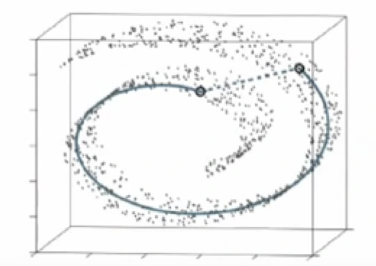
The PCA maximizes variance while t-SNE(solid line) preserves small distances.
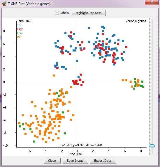
What is the t-SNE Plot?
The t-SNE plot is a dimensionality reduction technique that uses graphs to simplify large, high-dimension data. The t-SNE plot can use up a lot of CPU and memory when the number of probes increases. So it’s a good idea to use the plot only when the number of probes is not more than two thousand.
The Use Cases For The t-SNE Algorithm
t-SNE is used on almost all high-dimensional data sets. Python t-SNE is growing in prominence and has widespread applications in latest technologies Natural Language Processing (NLP), speech processing, image processing, and genomic data.
Other areas that t-SNE is used are cyber security, bioinformatics, and cancer research. t-SNE is also used to learn, investigate, and evaluate segmentation. However, since t-SNE does not preserve inputs like PCA, and values can change between runs, it is more a tool for exploration rather than a clustering approach. Here are some t-SNE Python examples.
Comparison of text using word vector representations
Word vector representations can capture both semantic concepts as well as linguistic properties (eg. tense, gender, singular/plural). Using Python t-SNE, a map in two dimensions can be created. In this map words that are semantically similar are placed close to one another. This allows one to have a top-down view of things like text summaries and source material, and text sources. As a result, users can even explore text sources like maps to identify patterns.
(i) Medical Imaging
Mass Spectrometry Imaging (MSI) is a relatively new technology that uses the t-SNE algorithm. MSI provides the spatial distribution for several biomolecules simultaneously. Using t-SNE, a non-linear data visualization is possible. This helps to resolve the biomolecular inratumour heterogenity issue.
In other words, t-SNE helps uncover tumour subpopulations linked to the survival of patients with gastric cancer. It also helps uncover metastasis status in breast cancer tumours. t-SNE clustering helps to provide useful and significant results in this scenario.
(ii) Facial Expression Recognition
Facial Expression Recognition(FER) application is one of the best t-SNE Python examples. It is especially challenging because the dimension reduction is complex and PCA is not adequate. Python t-SNE is used in FER with good results. It reduces high-dimensional data into a two-dimensional subspace. After this, other algorithms like NNs, Random Forests, Logistic Regression, etc are used for the expression classification.
Implementation Of The t-SNE Algorithm In Python
Installing the t-SNE package is not recommended in Python. It is better to access the t-SNE algorithm from the t-SNE sklearn package. The example below is taken from the t-SNE sklearn examples on the sklearn website.
## importing the required packages
from time import time
import numpy as np
import matplotlib.pyplot as plt
from matplotlib import offsetbox
from sklearn import (manifold, datasets, decomposition, ensemble,
discriminant_analysis, random_projection)
## Loading and curating the data
digits = datasets.load_digits(n_class=10)
X = digits.data
y = digits.target
n_samples, n_features = X.shape
n_neighbors = 30
## Function to Scale and visualize the embedding vectors
def plot_embedding(X, title=None):
x_min, x_max = np.min(X, 0), np.max(X, 0)
X = (X – x_min) / (x_max – x_min)
plt.figure()
ax = plt.subplot(111)
for i in range(X.shape[0]):
plt.text(X[i, 0], X[i, 1], str(digits.target[i]),
color=plt.cm.Set1(y[i] / 10.),
fontdict={‘weight’: ‘bold’, ‘size’: 9})
if hasattr(offsetbox, ‘AnnotationBbox’):
## only print thumbnails with matplotlib > 1.0
shown_images = np.array([[1., 1.]]) # just something big
for i in range(digits.data.shape[0]):
dist = np.sum((X[i] – shown_images) ** 2, 1)
if np.min(dist) < 4e-3:
## don’t show points that are too close
continue
shown_images = np.r_[shown_images, [X[i]]]
imagebox = offsetbox.AnnotationBbox(
offsetbox.OffsetImage(digits.images[i], cmap=plt.cm.gray_r),
X[i])
ax.add_artist(imagebox)
plt.xticks([]), plt.yticks([])
if title is not None:
plt.title(title)
#———————————————————————-
## Plot images of the digits
n_img_per_row = 20
img = np.zeros((10 * n_img_per_row, 10 * n_img_per_row))
for i in range(n_img_per_row):
ix = 10 * i + 1
for j in range(n_img_per_row):
iy = 10 * j + 1
img[ix:ix + 8, iy:iy + 8] = X[i * n_img_per_row + j].reshape((8, 8))
plt.imshow(img, cmap=plt.cm.binary)
plt.xticks([])
plt.yticks([])
plt.title(‘A selection from the 64-dimensional digits dataset’)
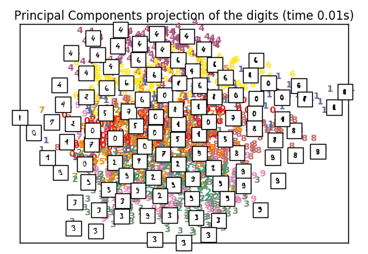
## Computing PCA
print(“Computing PCA projection”)
t0 = time()
X_pca = decomposition.TruncatedSVD(n_components=2).fit_transform(X)
plot_embedding(X_pca,
“Principal Components projection of the digits (time %.2fs)” %
(time() – t0))
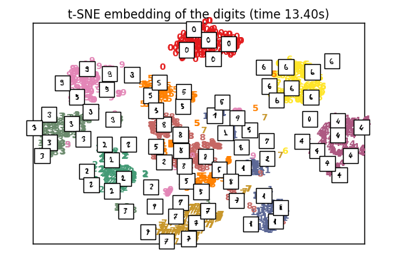
## Computing t-SNE
print(“Computing t-SNE embedding”)
tsne = manifold.TSNE(n_components=2, init=’pca’, random_state=0)
t0 = time()
X_tsne = tsne.fit_transform(X)
plot_embedding(X_tsne,
“t-SNE embedding of the digits (time %.2fs)” %
(time() – t0))
plt.show()
Time taken for implementation
t-SNE: 13.40 s
PCA: 0.01 s
Conclusion
t-SNE python is one of those algorithms that has shot into prominence of late. t-SNE Python examples abound in the industry as it is being used in cutting-edge technologies like NLP, medical imaging, and genomic data.
While PCA is similar to t-SNE in its use, there are some unique limitations and advantages of both algorithms. It’s a good idea for data science and machine learning enthusiasts to have an understanding of both.
Are you also inspired by the opportunities provided by Python? You may also enroll for a Python Programming Course for more lucrative career options in Data Science using Python.