Know Everything About Vlookup and Hlookup in Excel

Hlookup and Vlookup are functions in Excel that allow you to use a section of your spreadsheet as a lookup table.

Electronic Documents in the tabular form are often called a spreadsheet. In these specific types of documents or spreadsheet data is divided into cells. In each of these calls may contain a value in the numerical or text form that defines its presence in the sheet. This spreadsheet software also allows different formulas based out of these cells to get desired results.

Modern spreadsheet software is almost used in every office for its effectiveness in securing data in custom forms.

Almost more than 1+ Billion people are using this excel software daily(source). These can even store graphical forms inside the cells too.

Many top companies for spreadsheet software include Microsoft excel, Openoffice, Google Sheets and many more. These sheets nowadays come up with around 400+ features that are used within sheets. Here in this blog, we are going to use one of the most popular spreadsheet software Microsoft excel for example in studying the Vlookup and Hlookup function.

Though Logic remains the same for all spreadsheet software only the syntax gets changed. The formula of vlookup and hlookup, their syntax and difference between these two.

Here is a simple video explaining Vlookup and Hlookup in Excel

One of the main functions found in spreadsheet software is the Lookup function that is used to find specific values in a specific column or row. It is used mainly in two ways either Horizontally or Vertically.

When Horizontal values are to be searched that it is termed as Hlookup and simultaneously for vertical values is called as Vlookup. Although the difference between vlookup and hlookup are minor still they have are high values for the learning curve in excel.

Let’s study them with an example, syntax, and difference for vlookup and hlookup in excel.

Defining the Vlookup Function in Excel

Vlookup stands for Vertical Search, is used as a set of Lookup functions to define the value from a specific column in a table.

Syntax for vlookup

General Syntax for Vlookup Function is:

VLOOKUP(lookup_value, table_array, col_index_num, [range_lookup])

And say for example we have this table

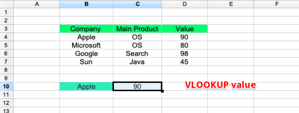
And we are looking for the value of the company Apple in the table. Here is the real formula for Vlookup function for this example. VLOOKUP(B10,B3:D7,3,FALSE)

where values are defined as:

lookup_value (required) = It is the main value that needs to be found in the table_array. This value must be inside the first column in the table range of cells defined in the table_array. For instance, in case the table_array has a span from B3:D7 then the lookup_value has to be inside the column B. This Lookup_value may be present in the form of value, a text string or a reference to a corresponding call. Here in the above example, we are looking for the Apple quantity in the given table.

table_array (required) = It is the range of the data Vlookup function will search for the lookup_value. Let us say for example data are listed in the range from B3:D7 than as described above lookup_values need to be in the B3 column to get the desired result.

col_index_num (required) = It defines the column that contains the return value. In this case, the leftmost column in the table_array is assigned number 1 and so on. For example in the range of B3:F6 the col_index_num, Column B will be 1, Column C as 2, Column D as 3 and so on. So for the above example, we are looking for the values of Apple in the above data in the D column.

range_lookup (optional) = Another parameter although optional it specifies whether you want the desired value to be matched as either Exact or Approximate.

Approximate Match: (1/True) This option searches for the value that corresponds to the closest value assuming the table is sorted either numerically or alphabetically in a specific order.

VLOOKUP(B10,B3:D7,3,False)

Here are some more practical examples for this function

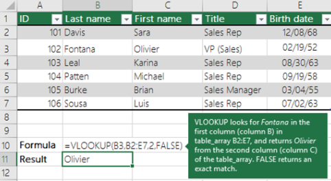
(i) Lookup_Value B3 is Fontana
(ii) Table array range from B2 to E7
(iii) Col is 2 so the value has to be inside the column C
(iv) False asks for an exact match

So we are looking for a person with the last name as Fontana and the corresponding answer we get inside the result column is Olivier.

Note: The first three values are required for Vlookup formulas to work in the excel. Whereas the fourth values are optional with wild characters also applicable based on approximate match conditions.

One has to put specific values inside a cell to get the desired results. Here are notable things you should know about Vlookup function.

(i) For Vlookup function to have more effective use absolute references for range_lookup so that looks for exact values always.

(ii) With Vlookup you can search both approximate and exact match queries along with wildcard(*) to get partial match answers for the respective function.

(iii) By default, to Vlookup function to work; Lookup value must be present in the first column of the table array and searchable data columns to the right.

(iv) Vlookup is used for data that are preferably organized in vertical rows so each row has specific new values in their cell.

(v) To get effective results from approximate match mode you must rearrange the data in ascending order.

(vi) Vlookup functions are case insensitive when in use so whether you APPLE, ApplE, or aPPLe it will search for Apple only.

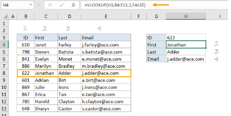
(vii) Vlookup follows the path from left to right to retrieve the results from a given value of the table. Assuming leftmost column as 1, then next as 2 and so on. You can check the below image to understand the column number used by Vlookup function.

(viii) If the values are not available in the data then Vlookup function will cause #N/A error. And you can also use the IFNA function to include a friendly message in the result with such as ‘Not Found’ to let the user know there is no value match for this data.

(ix) For Vlookup function, one must ensure data in the subsequent first column do not have any trailing spaces, quotation marks, leading spaces, or any nonprinting characters. This might lead to getting unexpected results from the use of Vlookup function in excel.

Common Errors Found in Vlookup Function Use

Wrong Value Returned

This specific value is seen as the range_lookup is avoided or default set to be TRUE and the first column is not sorted resulting in wrong value. So you have to either sort the first column or subsequent use of FALSE value to match exactly in the given table.

#REF in the Result Cell

This specific error is seen when the col_index_number is found to be higher or greater than the respective number of columns in the table_array then #REF will be seen in the outcome.

#Value in the Result Cell

This specific error comes when the table_array values are less than 1 then #value will come in the outcome.

#NAME? In the Result Cell

This specific error implies that your formula is missing the use of quotes in a person’s name.

#SPILL in the Result Cell

This specific spill error implies that your formula is using an entire column as a reference in the function.

Defining Hlookup Function in Excel

Hlookup stands for Horizontal Search, is a set of Lookup functions used for defining value from a specific row in the table.

Syntax for Hlookup

HLOOKUP( lookup_value, table_array, row_index_num, [range_lookup] )

Here is the example for the Hlookup function

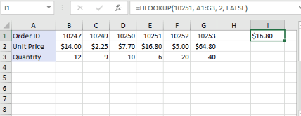
In the above image, we are looking to find the price value with order ID 10251 and from the second row to have an exact match. Here is the syntax for the Hlookup formula in excel.

HLOOKUP(10251, A1:G3, 2, FALSE) and it gives the result as $16.80 to have the desired result using this horizontal search function in excel.

Where parameters of the formula are:

lookup_value = First is the value the function should search for inside the table. In the above example, it is the ID 10251 that the Hlookup function will search inside the first row of the table. Depending on your data this value can be text or number but not any erroneous character.

table_array = It is again the range of the data that function will search in the given sheet. In the corresponding example, the Hlookup function will search for the value of 10251 coming from A1 to G3 range respectively.

row_index_num = As the name suggests it defines the row number from where the data is to be searched for. As in the above example row 1 is for the order ID and 2 is for Unit price. You can see we have used 2 to get the desired unit price value. As Hlookup function now is searching for 10251 value in the range from A1 to G3 in row 2.

[range_lookup] = Another important thing is to add the match value to be exact or approximate. These values are assigned as TRUE or False respectively. As we have added False so the Hlookup function is looking for an Exact match for the corresponding values of 10251 in the range of A1 to G3 inside row number 2. That value is $16.80 in the cell A2-G2.

Exact Match = With the exact match, we use FALSE in the Hlookup function in excel. Here in the above example we have used HLOOKUP(10251, A1:G3, 2, FALSE) and result found to be $16.80. If the values are not found exact then the result would be #N/A respectively.

Approximate Match = For approximate match we use TRUE in the Hlookup function and if the values are not found then it takes the nearest value to get the answers.

Here are some other notable things to know about the Hlookup function in excel.

(i) Lookup values for the Hlookup function are found by matching the first row of the table.

(ii) Hlookup like Vlookup also supports approximate, exact, and wildcards for finding values with partial match.

(iii) range_lookup defines the value for an exact or approximate match in Hlookup function.

(iv) So for an exact match set the range_lookup to be FALSE.

(v) For range_lookup is set TRUE, Hlookup function will match the nearest value less than the original one.

(vi) If range_lookup is not used or omitted then the Hlookup function will first look for an exact match then take the nearest values to get the result.

(vii) For range_lookup FALSE or the Exact match values of the first row don’t require sorting.

(viii) For range_lookup TRUE or the approximate match, the lookup values need to be sorted out first otherwise you will get an incorrect answer from the function.

Now we are going to have a look at the formula of vlookup and hlookup with their precise syntax.

The Formula of Vlookup and Hlookup Functions

Both Vlookup and Hlookup have a specific formula that one must enter to get the desired results.

Syntax for the formula of Vlookup and Hlookup

For Vlookup

VLOOKUP(lookup_value, table_array, col_index_num, [range_lookup])

For Hlookup

HLOOKUP( lookup_value, table_array, row_index_num, [range_lookup])

It is to be noted that when values are in the first row of a given table than Hlookup is used whereas if the values are in the first column of a table then the Vlookup is preferred.

Although it seems confusing for beginners but for individuals dealing with these formulas on a daily basis their use is quite straightforward and takes a different path altogether. And if you are looking for a job that requires Excel proficiency then one must master these two searching functions (vlookup and hlookup in excel).

Difference between Vlookup and Hlookup in Excel

Both functions are used to find specific values in the data with Vlookup search with vertical columns while the Hlookup searches within horizontal rows.

Here are the main difference between Vlookup and Hlookup functions in excel:

(i) Hlookup functions though has a lot of importance in finding the values in a given table but in a practical world most of the data are available in the vertical rows. Hence Vlookup is more frequently used than the Hlookup function in real-time.

(ii) Hlookup function by default starts to search the value inside the top row of a given table and then returns the corresponding value inside the same column only. Whereas Vlookup functions search the value from the column and then interprets the result in the next column of the same row.

(iii) The pre-requisite for the Hlookup function is that searchable value or range must be inside the topmost column of a given table. While in Vlookup function the value has to be inside the leftmost column of the given table or range.

Conclusion

Here we can conclude that both Vlookup and Hlookup are part of the excel functions used to define specific values in the spreadsheet. Vlookup is used for finding vertical values in the data table whole Hlookup is used to find values through horizontal checks in the data table. Both formulae of vlookup and hlookup have similarities with the major difference between row and column values.

MS Excel is among the most spreadsheet sheet software encouraging data to be stored in a tabular form. Although when the data are small the values can be obtained just by having a look around. These functions become highly useful for Businesses with a huge amount of data and if one is looking for approximate or exact value in millions of data then these functions are your first choice.

As most of the time, we see data sheets in excel are more vertically defined or they store more data in the vertical alignment so Vlookup is used more in comparison to Hlookup. Though horizontal values may have the same significance too. To be a professional in excel, you must have the right learning curve to understand the difference between vlookup and hlookup function in general.

So, if you are also planning to build your career in data analytics to the next level, then you should enroll in the Certified Data Analytics Course.