Introduction
Want to surf the road of Linear Regression? Learn the variant Linear Regression Formulas in this post and get a knowledgeable insight into Linear Regression map. Artificial Intelligence has become ubiquitous these days. People across various different disciplines are trying to use AI to make their tasks a lot easier and more efficient.
To give you a brief idea about it, doctors are using AI to classify whether a tumor is malignant or benign, HR recruiters use AI to check resume of applicants to verify if they meet the minimum criteria for job, economists use AI to predict future movements of market, meteorologists use AI to predict the weather, and so on. The thrust behind such prevalent use of AI is machine learning algorithms.
Do you know a PwC report estimates the contribution of the AI industry to 15.7 trillion U.S. Dollars by 2030. That is huge. The rudimentary algorithm to start within machine learning is the linear regression. Hence, if you want to learn ML algorithms but haven’t got your feet wet yet, you are in the right place.
In this post, I will cover all the linear regression formulas, which include hypothesis, cost function, gradient descent and the equation of prediction interval as well. If you want a detailed look at how linear regression works, look through this post Tutorial of Python Linear Regression first.
What is linear regression
For those completely new to machine learning, let me first give you a brief idea about linear regression. And even before knowing what linear regression is, let us get ourselves accustomed to regression. Regression is a technique of modelling a target value based on independent predictors. It is mostly used for forecasting and finding the relationship between variables.
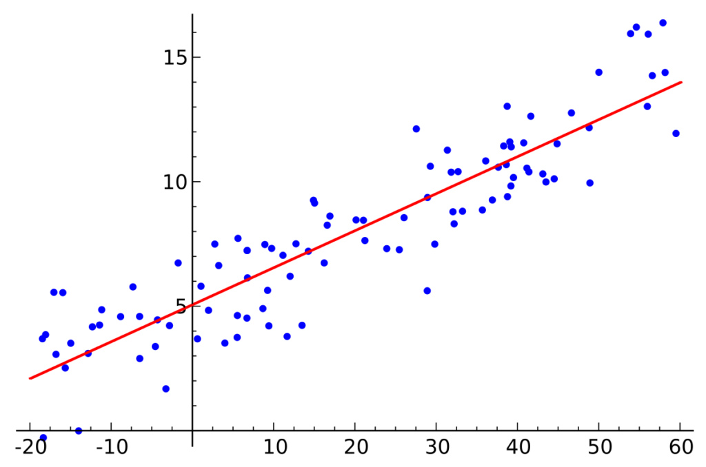
Simple linear regression is one type of regression technique where the number of independent variables is one and the relationship between the dependent(y) and independent(x) variable is a linear relationship.
Linear regression equation formula
Y = theta0 + theta1(x1)
Where theta0 and theta1 are called parameters. Before moving on let us understand two more equations which you must know to better understand linear regression.
Cost function
The idea behind the cost function is that we choose the values of theta0 and theta1 such that the h(x), our hypothesis or you can say the output of the function, is close to y— output variable— for our training example (x, y). The cost function is also called Squared error function.
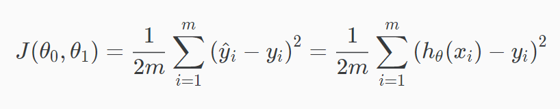
The equation is as shown above. Also, please note that m= number of the training set and ½ is taken for the sake of simplicity in the calculation for the later stage.
Gradient descent
The next concept you need to understand is gradient descent. It is a method of updating theta0 and theta1 to reduce the cost function or cost of the function. The main idea lies behind starting with some values for theta0 and theta1 and then changing those values iteratively to reduce the cost. It helps us on how to change values.
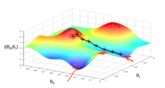
To draw an analogy, imagine you are standing on a mountain and your goal is to reach the bottom of the mountain. There is a catch though. You can only take the discrete number of steps to reach to the bottom. If you decide to take one step at a time, it would take a longer time. And If you choose to take longer steps, you may reach sooner but you may overshoot the bottom and reach to the point that is not exactly the bottom. This, the number of steps you take is the learning rate. This decides how fast the algorithm converges to the minimum.
You must be wondering how to use gradient descent to update theta0 and theta1, right? Let’s get to it. To update both, theta0 and theta1, we take gradients from the cost function. To find these, we take partial derivatives with respect to theta0 and theta1. Now, to understand partial derivatives you require some calculus but if you don’t, take it as it is, it’s totally alright.
Gradient descent linear regression formula
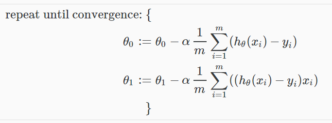
As you can see, alpha is our learning rate and followed by that the partial derivative is the gradients which are used to update values of theta0 and theta1. A smaller learning rate could get you closer to local minima but takes more time to reach the minimum, whereas a larger learning rate converges sooner but there is a chance that you could overshoot the minimum.
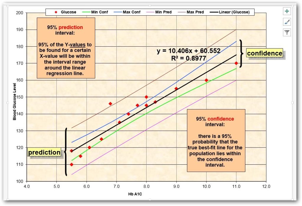
Another useful technique— Prediction Intervals
Our regression model generates values which are estimates. Different models generate different outcomes. That’s where Prediction intervals really help. In general, it draws out and intervals as the name suggests. It is the most commonly used technique in regression statistics, but may also be used with normally distributed data. And the calculation of a prediction interval for normally distributed data is much simpler than that required for regressed data.
Confidence interval and Prediction interval formula linear regression
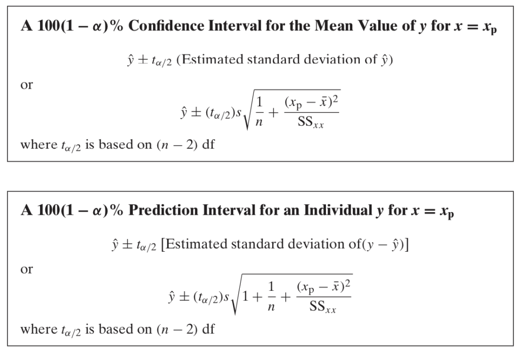
Confidence intervals that only concerned with the center of the distribution, whereas prediction intervals consider the tails of the distribution as well as the center. As a result, prediction intervals have a much greater sensitivity to the assumption than do confidence intervals. Therefore, the assumption of normality should be tested prior to calculating a prediction interval.
Things to take care of
While performing linear regression there are several things you should take care of. To start with, outliers and influential observations. A point that is far from the linear regression prediction line is known as an outlier and that can affect our results. Another thing is residuals, which is a feature rather than a flaw. After the model has been implemented, plotting the residuals on the y-axis against the variable on the x-axis reveals any possible non-linear relationship among the variables.
A lurking variable is also a concern worth addressing. It exists when the relationship between two of the variables is significantly affected by the presence of a third variable that has not been included in the modelling effort.
Endnotes
With the availability of series of algorithms to choose from, Linear Regression is an algorithm that every enthusiast of Machine Learning must know and also it is the right place to start for the people who want to learn Machine Learning as well. It is a simple but useful algorithm. Start Learning today and if you have any doubts let us know in the comment section below, we’ll guide you through all your queries. Happy Learning.